
The Problem: I spent five years in a PhD program learning how to formulate optimization problems. Sensor selection, supply chain design, resource allocation — all of it was about taking a real-world decision and encoding it as a mathematical model that a solver could handle.
Then I took a data engineering job. And for the first time, I was building the plumbing — the pipelines, the orchestration, the monitoring — rather than the brain. The models existed. Someone else trained them. I just moved the data around and made sure the DAGs didn’t break.
That felt wrong. Not because data engineering is unimportant (it’s not — a model without reliable data is a toy). But because the part of my brain that lights up when I’m reasoning about trade-offs, constraints, and objective functions was sitting idle.
So I built a project that sits at the intersection of both: a system where machine learning produces the input for an optimization solver, and the whole thing runs as a production pipeline with monitoring, retraining, and a live API.
This is how I built it.
The Architecture in One Sentence
Forecast demand per zone per day (ML) → solve a capacitated vehicle routing problem with time windows (OR) → serve the result (API) → monitor for drift (MLOps) → retrain if needed (automation).
┌─────────────────────────────────────────────────────────────┐
│  GitHub Actions (daily, 06:00 UTC)                          │
│                                                             │
│  1. Ingest ──▶ 2. Forecast ──▶ 3. Solve ──▶ 4. Drift Check │
│  NYC TLC data    LightGBM       OR-Tools CVRP-TW    PSI     │
│               + PyTorch LSTM   (haversine)            │     │
│                                                             │
│  If PSI > 0.25 ──▶ Retrain ──▶ Re-solve ──▶ Commit         │
└─────────────────────────────────────────────────────────────┘
                         │
                         ▼
┌─────────────────────────────────────────────────────────────┐
│  Render (always-on)                                         │
│  FastAPI: /forecast  /routes  /predict  /health             │
└─────────────────────────────────────────────────────────────┘
Why VRP? Why Not a “Boring” Classification Problem?
Most ML portfolio projects are: load a CSV, train a model, report accuracy. That’s fine for a first project. But it doesn’t demonstrate the full MLOps lifecycle.
The Vehicle Routing Problem is:
- Genuinely hard (NP-hard, no exact solution for realistic instances)
- Where ML actually adds value (demand forecasting changes the solver’s input, which changes the output)
- Where optimization background matters (you need to understand what the solver is doing to debug it, not just call it)
- Visually compelling (routes on a map beat a confusion matrix)
- The hybrid “ML forecast → OR solve” pattern is well-represented in 2025–2026 literature and is exactly the architecture that logistics companies (Amazon, FedEx, UPS) use in production.
The Data
I used 6 months of NYC Yellow Taxi trip records (public, ~1.6B trips total). I aggregated them to zone-day trip counts for 18 zones in Manhattan/Bronx. This gives me:
A real time series with seasonality, day-of-week effects, and spatial correlation A realistic demand distribution (3–558 trips per zone per day) Zone geometry (lat/lon centroids) for computing real distances The zones come from the official TLC shapefile. I computed centroids with geopandas and used haversine (great-circle) distances between zone centers. This is a documented simplification — production systems use road-network travel times (OSRM, GraphHopper). For a 18-zone instance, the difference is small enough that it doesn’t change the solver’s decisions.
The Forecasting Layer
I trained two models on the same features (lag-1, lag-7, 7-day rolling mean/std, day-of-week, is-weekend):
| Model | Architecture |
|---|---|
| LightGBM | 300 trees, depth 6, lr=0.05 |
| PyTorch LSTM | 2 layers, 128 hidden, dropout 0.1 |
Here is a chart displaying MAE for both the models
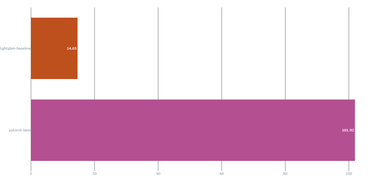
LightGBM won. On tabular time-series data with ~2000 training samples per zone, gradient boosting is hard to beat. The LSTM is retained in the codebase for ablation and potential ensemble use, and it’s logged in MLflow alongside the GBM so the comparison is reproducible.
This is an important lesson I want to be honest about: the neural net was not better.
The Optimization Layer
The solver is OR-Tools (Google’s open-source constraint programming library) solving a CVRP-TW (Capacitated Vehicle Routing Problem with Time Windows):
- 18 locations (17 zones + 1 depot)
- 20 vehicles, each with a capacity constraint
- Time windows: each zone must be visited between 5 AM and 8 PM
- Objective: minimize total route distance
The key design decision: demand from the ML forecast becomes the node weight in the VRP. A zone forecast to have 500 trips needs more vehicle capacity than a zone forecast to have 30. The solver routes accordingly.
This is where the ML and OR actually interact — not just “ML model exists” and “OR solver exists” in the same repo, but the ML output changes the optimization result.
The Serving Layer
FastAPI on Render (free tier, 512 MB RAM). Three endpoints:
- GET /forecast — returns the latest per-zone forecast (pre-computed by the daily pipeline)
- GET /routes — returns the latest solved routes
- POST /predict — live single-point inference (pass features, get a forecast in ~15 ms)
- The /predict endpoint is the one that makes it feel like a “real ML system” rather than a “JSON file server.” Anyone can open /docs, POST some features, and get a number back in real time.
Why Render and not FastAPI Cloud? FastAPI Cloud (the fastapi deploy CLI) doesn’t support custom system dependencies. LightGBM needs libgomp1 (GNU OpenMP runtime), which isn’t in FastAPI Cloud’s base image. Render uses your Dockerfile, so you can apt-get install libgomp1 in the build step.
The MLOps Layer
Daily Pipeline (GitHub Actions, 06:00 UTC)
Ingest → Features → Train → Solve → Drift Check → (Retrain if needed) → Commit
The pipeline commits its outputs (forecast.json, routes.json, drift.json, lightgbm_model.txt) to the repo. The Render deployment reads these files on each request. No redeployment needed — the API always serves the latest committed results.
Drift Monitoring Every day, the pipeline computes the Population Stability Index (PSI) between the model’s forecast and the actual demand over the last 7 days:
- PSI < 0.10 → stable (do nothing)
- PSI 0.10–0.25 → moderate drift (log a warning)
- PSI > 0.25 → significant drift → trigger a full retrain
The retrain is just… re-running the same pipeline. No special code. The if: contains(steps.drift.outputs, 'drift_detected') condition in the workflow YAML gates it.
Why PSI and not a KS test? PSI is more interpretable for multi-modal distributions (your demand has weekends and weekdays, which is bimodal). KS assumes a specific distributional form. PSI just compares bin proportions — no assumptions, well-established thresholds from the credit scoring industry.
The Dashboard
A Streamlit app (deployed on Streamlit Community Cloud, free) with three tabs:
- Routes on a map — Folium map with color-coded routes, zone markers, and total distance
- Forecast accuracy — Daily MAE over time + per-zone forecast vs. actual bar chart
- Drift — Current PSI value, status (stable/drift), and whether retrain was triggered
- Routes over real NYC geography, computed by a solver, fed by a forecast model.
What I Learned (the unglamorous part)
The solver is infeasible more often than you’d think.
I spent an entire day debugging why OR-Tools returned “no feasible solution.” It turned out to be a time-dimension span that was smaller than the time window upper bound. The solver doesn’t tell you which constraint is infeasible. You have to reason about it, In this case it was to look at the LP relaxation and figure out which constraint was binding.
The depot’s demand gets counted once per vehicle.
In a multi-vehicle VRP, the depot is visited by every vehicle. If the depot has non-zero demand, it consumes N × depot_demand total capacity. I had 10 vehicles and a depot with 128 demand → 1280 capacity consumed before any real zone was visited. Zeroing the depot’s demand fixed it.
to_json silently corrupts your dates.
Pandas to_json converts datetimes to epoch integers. read_json gives you integers back. pd.to_datetime interprets them as nanoseconds since epoch → 1970-01-01. My drift monitoring was comparing 1970 dates against 2025 dates for a week before I noticed.
512 MB is enough. If you don’t load PyTorch.
The entire FastAPI service (LightGBM model + OR-Tools + Uvicorn) runs in ~200 MB. PyTorch’s import alone is 300+ MB. The lesson: your serving stack should be the minimal set of dependencies needed for inference. Training happens in the pipeline (GitHub Actions, 16 GB RAM). Serving happens in the API (512 MB). They’re different environments.
uv changed how I think about dependency management.
uv lock + uv sync –frozen is the first time I’ve had truly reproducible installs across local, CI, and Docker without a 200-line requirements.txt that breaks every time a transitive dependency updates. The lock file is the contract.
What’s Next
- Road-network distances (OSRM/GraphHopper) instead of haversine
- Dynamic re-optimization (a new order arrives at 10 AM → re-solve with updated demand)
- Ensemble forecasting (average LightGBM + LSTM, or use the LSTM residual as a feature for the GBM)
- Larger instance (all 263 NYC zones, partitioned by borough)
- RL for the routing policy (not to replace OR-Tools, but to learn a fast heuristic for the initial solution that OR-Tools then improves)
Links
- Code: github.com/Amol-Kulkarni91/ml-vrp
- Live API: ml-vrp.onrender.com/docs
- Dashboard: link
