
A new look at an old research study
In 1986, a group of urologists in London published a research paper in The British Medical Journal that compared the effectiveness of two different methods to remove kidney stones. Treatment A was open surgery (invasive), and treatment B was percutaneous nephrolithotomy (less invasive). When they looked at the results from 700 patients, treatment B had a higher success rate. However, when they only looked at the subgroup of patients different kidney stone sizes, treatment A had a better success rate. What is going on here? This known statistical phenomenon is called Simpson’s paradox. Simpson’s paradox occurs when trends appear in subgroups but disappear or reverse when subgroups are combined. In this project we are going to explore Simpson’s paradox using multiple linear regression and other statistical tools. The data used for this project can be found here.
# Load the readr and dplyr packages
library(readr)
library(dplyr)

# Read datasets kidney_stone_data.csv into data
data <- read_csv("kidney_stone_data.csv")

# Take a look at the first few rows of the dataset
head(data)
| treatment | stone_size | success |
|---|---|---|
| B | large | 1 |
| A | large | 1 |
| A | large | 0 |
| A | large | 1 |
| A | large | 1 |
| B | large | 1 |
Recreate the Treatment X Success summary table
The data contains three columns: treatment (A or B), stone_size (large or small) and success (0 = Failure or 1 = Success). To start, we want to know which treatment had a higher success rate regardless of stone size. We will create a table with the number of successes and frequency of success by each treatment using the tidyverse syntax.
# Calculate the number and frequency of success and failure of each treatment
data %>%
  group_by(treatment, success) %>%
  summarise(N = n()) %>%
  mutate(Freq = round(N/sum(N), 3))
| treatment | success | N | Freq |
|---|---|---|---|
| A | 0 | 77 | 0.22 |
| A | 1 | 273 | 0.78 |
| B | 0 | 61 | 0.174 |
| B | 1 | 289 | 0.826 |
Bringing stone size into the picture
From the treatment and success rate descriptive table, we saw that treatment B performed better on average compared to treatment A (82% vs. 78% success rate). Now, we shall consider stone size and see what happens. We are going to stratify the data into small vs. large stone subcategories and compute the same success count and rate by treatment like we did in the previously.
The final table will be treatment X stone size X success.
# Calculate number and frequency of success and failure by stone size for each treatment
sum_data <-
  data %>%
  group_by(treatment, stone_size, success) %>%
  summarise(N = n()) %>%
  mutate(Freq = round(N/sum(N), 3))

# Print out the data frame we just created
print(sum_data)
| treatment | stone_size | success | N | Freq |
|---|---|---|---|---|
| A | large | 0 | 71 | 0.27 |
| A | large | 1 | 192 | 0.73 |
| A | small | 0 | 6 | 0.069 |
| A | small | 1 | 81 | 0.931 |
| B | large | 0 | 25 | 0.312 |
| B | large | 1 | 55 | 0.688 |
| B | small | 0 | 36 | 0.133 |
| B | small | 1 | 234 | 0.867 |
When in doubt, rely on a plot
What is going on here? When stratified by stone size, treatment A had better results for both large and small stones compared to treatment B (i.e., 73% and 93% v.s. 69% and 87%). Sometimes a plot is a more efficient way to communicate hidden numerical information in the data.
# Load ggplot2
library(ggplot2)

# Create a bar plot to show stone size count within each treatment
sum_data %>%
  ggplot(aes(x = treatment, y = N)) +
  geom_bar(aes(fill = stone_size), stat="identity")

Identify and confirm the lurking variable
From the bar plot, we noticed an unbalanced distribution of kidney stone sizes in the two treatment options. Large kidney stone cases tended to be in treatment A, while small kidney stone cases tended to be in treatment B. We can confirm this hypothesis with statistical testing.
We will analyze the association between stone size (i.e., case severity) and treatment assignment using a statistical test called Chi-squared. The Chi-squared test is appropriate to test associations between two categorical variables. This test result, together with the common knowledge that a more severe case would be more likely to fail regardless of treatment, will shed light on the root cause of the paradox.
# Load the broom package
library(broom)

# Run a Chi-squared test
trt_ss <- chisq.test(data$treatment, data$stone_size)

# Print out the result in tidy format
print(trt_ss)
	Pearson's Chi-squared test with Yates' continuity correction

data:  data$treatment and data$stone_size
X-squared = 189.36, df = 1, p-value < 2.2e-16
Remove the confounding effect
After the above test, we are confident that stone size/case severity is indeed the lurking variable (aka, confounding variable) in this study of kidney stone treatment and success rate. The good news is that there are ways to get rid of the effect of the lurking variable.
We will be using multiple logistic regression to remove the unwanted effect of stone size, and then tidy the output with a function from the broom package.
# Run a multiple logistic regression
m <- glm(data = data, success ~  treatment + stone_size, family = "binomial")

# Print out model coefficient table in tidy format
tidy(m)
| term | estimate | std.error | statistic | p.value |
|---|---|---|---|---|
| (Intercept) | 1.03 | 0.134 | 7.68 | 1.55E-14 |
| treatmentB | -0.357 | 0.229 | -1.56 | 1.19e- 1 |
| stone_sizesmall | 1.26 | 0.239 | 5.27 | 1.33e- 7 |
Visualize model output
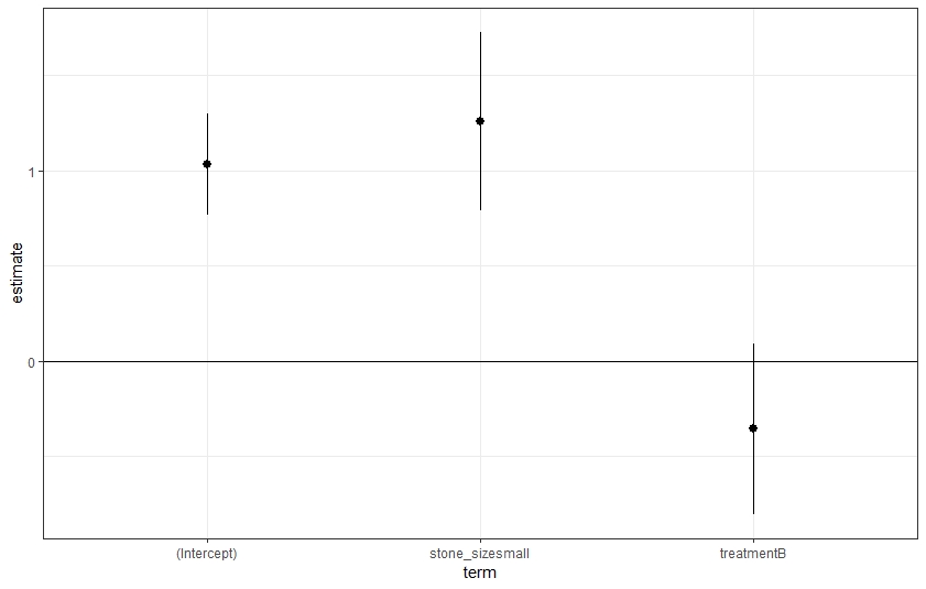
We successfully fit a multiple logistic regression and pulled out the model coefficient estimates! Typically (and arbitrarily), P-values below 0.05 indicate statistical significance. Another way to examine whether a significant relationship exists or not is to look at the 95% confidence interval (CI) of the estimate. In our example, we are testing to see:
- if the effect of a small stone is the same as a big stone, and
- if treatment A is as effective as treatment B.
If the 95% CI for the coefficient estimates cover zero, we cannot conclude that one is different from the other. Otherwise, there is a significant effect.
# Save the tidy model output into an object
tidy_m <- tidy(m)

# Plot the coefficient estimates with 95% CI for each term in the model
tidy_m %>%
  ggplot(aes(x = term, y = estimate)) +
  geom_pointrange(aes(ymin = estimate - 1.96 * std.error,
                      ymax = estimate + 1.96 * std.error)) +
  geom_hline(yintercept = 0) + theme_bw()
Conclusion
A coefficient represents the effect size of the specific model term. A positive coefficient means that the term is positively related to the outcome. For categorical predictors,the coefficient is the effect on the outcome relative to the reference category. In our study, stone size large and treatment A are the reference categories. Based on the coefficient estimate plot and the model output table, there is enough information to draw the following conclusions
- Small stone is more likely to be a success after controlling for treatment option effect
- Treatment A is not significantly better than B