We want to model infectious diseases. These diseases can spread from one member of a population to another; we try to gain insights into how quickly they spread, what proportion of a population they infect, what proportion dies, etc. One of the easiest ways to model them (and the way we’re focusing on here) is with a compartmental model. A compartmental model separates the population into several compartments, for example:
- Susceptible (can still be infected, “healthy”)
- Infected
- Recovered (were already infected, cannot get infected again)
That is, we might have a population of N=1000 (for example 1000 people) and we know that 400 people are infected at time t (for example t=7 days after outbreak of the disease). This is denoted by S(7) = 400. The SIR-Model allows us to, only by inputting some initial parameters, get all values S(t), I(t), R(t) for all days t. Let us consider the following example:
We have a new disease, disease X. For this disease, the probability of an infected person to infect a healthy person is 20%. The average number of people a person is in contact with per day is 5. So, per day, an infected individual meets 5 people and infects each with 20% probability. Thus, we expect this individual to infect 1 person (20% ⋅ 5 = 1) per day. This is $\beta$, the expected amount of people an infected person infects per day.
Now one can see that the number of days that an infected person has and can spread the disease is extremely important. We’ll call this number D. If D=7, an infected person walks around for seven days spreading the disease, and infects 1 person per day (because $\beta$=1). So we expect an infected person to infect 1⋅7 (1 per day times 7 days) = 7 other people. This is the basic reproduction number $R_0$, the total number of people an infected person infects. We just used an intuitive formula: $R_0 = \beta ⋅ D$.
We actually don’t need anything else, just one small notation: $\gamma$ will be 1/D, so if you think of D as the number of days an infected person has the disease, you can think of $\gamma$ as the rate of recovery, or the proportion of infected recovering per day. For example, if currently 30 people are infected and D=3 (so they’re infected for three days), then per day, 1⁄3 (so 10) of them will recover, so $\gamma$ =1⁄3. With $\gamma$ = 1/D, so D = 1/$\gamma$ , and $R_0 = \beta ⋅ D$, it follows that $R_0 = \beta/ \gamma$.
Here you can see the most important variables and their definitions again:
- N: total population
- S(t): number of people susceptible on day t
- I(t): number of people infected on day t
- R(t): number of people recovered on day t
- $\beta$: expected amount of people an infected person infects per day
- D: number of days an infected person has and can spread the disease
- $\gamma$: the proportion of infected recovering per day ($\gamma$ = 1/D)
- $R_0$: the total number of people an infected person infects ($R_0 = \beta/ \gamma$)
We now want to get the number of infected, susceptible and recovered for all days, just from $\beta, \gamma$ and N. Now, it is difficult to obtain a direct formula for S(t), I(t) and R(t). However, it is quite simple to describe the change per day of S, I, and R, that is, how the number of susceptible/infected/recovered changes depending on the current numbers. Again, we’ll derive the formulas by example:
We are now on day t after outbreak of disease X. Still, the expected amount of people an infected person infects per day is 1 (so $\beta$=1) and the number of days that an infected person has and can spread the disease is 7 (so $\gamma$=1⁄7 and D=7).
Let’s say that on day t, 60 people are infected (so I(t)=60), the total population is 100 (so N=100), and 30 people are still susceptible (so S(t)=30 and R(t)=100–60–30=10). Now, how do S(t) and I(t) and R(t) change to the next day?
We have 60 infected people. Each of them infects 1 person per day (that’s $\beta$). However, only 30⁄100 =30% of people they meet are still susceptible and can be infected (that’s S(t) / N). So, they infect 60 ⋅ 1 ⋅ 30⁄100 = 18 people (again, think about it until it really makes sense: 60 infected that infect on average 1 person per day, but only 30 of 100 people can still be infected, so they do not infect 60⋅1 people, but only 60⋅1⋅30/100 = 18 people). So, 18 people of the susceptibles get infected, so S(t) changes by minus 18. Plugging in the variables, we just derived the first formula:
Change of S(t) to the next day = - $\beta$ ⋅ I(t) ⋅ S(t) / N.
If you’re familiar with calculus, you know we have a term for describing the change of a function: the derivative S’(t) or dS/dt. (After we have derived and understood all the derivatives S’(t), I’(t) and R’(t), we can calculate the values of S(t), I(t) and R(t) for each day.)
So: S’(t) = - $\beta$ ⋅ I(t) ⋅ S(t) / N
Now, how does the amount of infected change? That’s easy: There are some new people infected, we just saw that. Exactly the amount of people that “leave” S(t) “arrive” at I(t). So, we have 18 new infected and we already know that the formula will be similar to this: I’(t) = $\beta$ ⋅ I(t) ⋅ S(t) / N (of course, we can omit the plus, it’s just to show you that we gain the exact amount that S(t) loses, so we just change the sign). There’s just one thing missing: some people recover. Remember, we have $\gamma$ for that, it’s the proportion of infected recovering per day.
We have 60 infected and $\gamma$=1⁄3, so one third of the 60 recovers. That’s 1⁄3 ⋅ 60 = 20. Finally, we obtain the formula:
I’(t) = $\beta ⋅ I(t) ⋅ S(t) / N -\gamma ⋅ I(t)$
The first part is the newly infected from the susceptibles. The second part is the recoveries.
Finally, we get to the last formula, the change in recoveries. The newly recovered are exactly the 20 we just calculated; there are no people leaving the “recovered”-compartment. Once recovered, they stay immune:
R’(t) = $\gamma$ ⋅ I(t)
Great, we have now derived all the formulas we need. We’ll now code and visualize an example model. Let’s import the necessary libraries and function to code the model.
from scipy.integrate import odeint
import numpy as np
import matplotlib.pyplot as plt
%matplotlib inline
We define the initial parameters for a disease. The scenario here is that the total population is 1000 and an infected person infects one other person per day. The infections last for four days.
N = 1000
beta = 1.0
D = 4.0
gamma = 1.0/D

s0, I0, R0 = 999, 1, 0 # initial conditions: one infected, rest susceptible
Let us write a function to code the different compartments of the model
def deriv(y, t, N, beta, gamma):
    S, I, R = y
    dSdt = -beta * S* I / N
    dIdt = beta * S * I / N - gamma * I
    dRdt = gamma * I
    return dSdt, dIdt, dRdt
We get our values S(t), I(t) and R(t) from the function odeint that takes the formulas we defined above, the initial conditions, and our variables N, $\beta$ and $\gamma$ and calculates S, I, and R for 50 days.
t = np.linspace(0, 50, 50) # Grid of time points (in days)
y0 = s0, I0, R0 # Initial conditions vector

#Integrate the SIR equations over the timegrid, t.
ret = odeint(deriv, y0, t, args = (N, beta, gamma))
S, I, R = ret.T
def plotsir(t, S, I, R):
    f, ax = plt.subplots(1, 1, figsize = (10,4))
    ax.plot(t, S, 'b', alpha = 0.7, linewidth = 2, label = 'Susceptible')
    ax.plot(t, I, 'y', alpha = 0.7, linewidth = 2, label = 'Infected')
    ax.plot(t, R, 'g', alpha = 0.7, linewidth = 2, label = 'Recovered')

    ax.set_xlabel('Time (days)')

    ax.yaxis.set_tick_params(length=0)
    ax.xaxis.set_tick_params(length=0)
    ax.grid(b=True, which = 'major', c = 'w', lw=2, ls='-')
    legend = ax.legend()
    legend.get_frame().set_alpha(0.5)
    for spine in ('top', 'right', 'bottom', 'left'):
        ax.spines[spine].set_visible(False)
    plt.show();
Now we just plot the result and arrive at this:
plotsir(t, S, I, R)
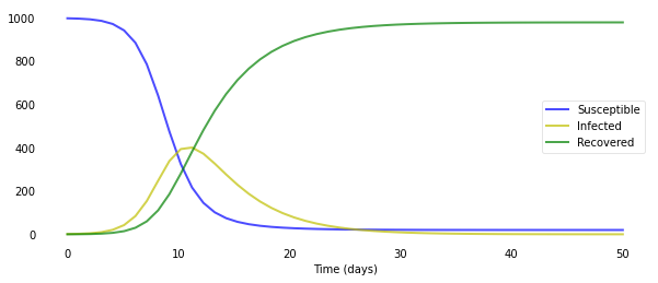
As you can see, it only takes around 30 days for almost a whole population of 1000 people to get infected. Of course, the disease modeled here has a very high $R_0$ value of 4.0. Just changing the number of people an infected person infects per day β to 0.5 results in a completely different scenario.
plotsir(t, S, I, R)
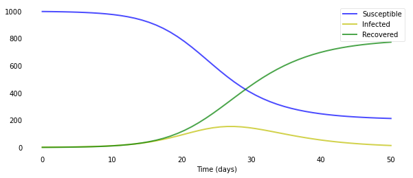
As you can see, these systems of ODEs are extremely sensitive to the initial parameters. That’s also why it’s so hard to correctly model an emerging outbreak of a new disease: we just do not know what the parameters are, and even slight changes result in widely different outcomes.
Introducing new Compartments
Many infectious diseases have an incubation period before being infectious during which the host cannot yet spread the disease. We’ll call such individuals — and the whole compartment — Exposed.
Intuitively, we’ll have transitions of the form S → E → I → R: Susceptible people can contract the virus and thus become exposed, then infected, then recovered. The new transition S → E will have the same arrow as the current S → I transition, as the probability is the same (all susceptibles can be exposed), the rate is the same (“exposition” happens immediately) and the population is the same (the infectious individuals can spread the disease and each exposes $\beta$ new individuals per day). There’s also no reason for the transition from I to R to change. The only new transition is the one from E to I: the probability is 1 (everyone that’s exposed becomes infected), the population is E (all exposed will become infected), and the rate gets a new variable, $\delta$. We arrive at these transitions:

From these transitions, we can immediately derive these equations
dS/dt = - $\beta$ . I . S/N
dE/dt = $\beta$ . I . S/N - $\delta$ . E
dI/dt = $\delta$ . E - $\gamma$ . I
dR/dt = $\gamma$ . I
Deriving the Dead-Compartment
For very deadly diseases, this compartment is very important. For some other situations, you might want to add completely different compartments and dynamics (such as births and non-disease-related deaths when studying a disease over a long time); these models can get as complex as you want!
When can people die from the disease? Only while they are infected! That means that we’ll have to add a transition I → D. Of course, people don’t die immediately; We define a new variable $\rho$ for the rate at which people die (e.g. when it takes 6 days to die, $\rho$ will be 1⁄6). There’s no reason for the rate of recovery, $\gamma$, to change. So our new model will look somehow like this:

The only thing that’s missing are the probabilities of going from infected to recovered and from infected to dead. That’ll be one more variable, the death rate $\alpha$. For example, if $\alpha$=5%, $\rho$ = 1 and $\gamma$ = 1 (so people die or recover in 1 day) and 100 people are infected, then 5% ⋅ 100 = 5 people will die. That leaves 95% ⋅ 100 = 95 people recovering. So all in all, the probability for I → D is $\alpha$ and thus the probability for I → R is 1-$\alpha$. We finally arrive at this model:

Which naturally translates to these equations:
dS/dt = - $\beta$ . I . S/N
dE/dt = $\beta$ . I . S/N - $\delta$ . E
dI/dt = $\delta$ . E - (1 - $\alpha$) . $\gamma$ . I - $\alpha . \rho$ . I
dR/dt = (1 - $\alpha$) . $\gamma$ . I
dD/dt = $\alpha . \rho$ . I
Let’s code the dead compartment -
def deriv(y, t, N, beta, gamma, delta, alpha, rho):
    S, E, I, R, D = y
    dSdt = -beta * S * I / N
    dEdt = beta * S * I / N - delta * E
    dIdt = delta * E - (1- alpha) * gamma * I - alpha *rho * I
    dRdt = (1- alpha) * gamma * I
    dDdt = alpha * rho * I
    return dSdt, dEdt, dIdt, dRdt, dDdt
We’ll model a highly infectious ($R_0$ = 5.0) disease in a population of 1 million, with an incubation period of 5 days and a recovery taking 7 days
N = 1_000_000
D = 4.0 # infections lasts four days
gamma = 1.0 / D
delta = 1.0 / 5.0  # incubation period of five days
R_0 = 5.0
beta = R_0 * gamma  # R_0 = beta / gamma, so beta = R_0 * gamma
alpha = 0.2  # 10% death rate
rho = 1/9  # 9 days from infection until death
S0, E0, I0, R0, D0 = N-1, 1, 0, 0, 0  # initial conditions: one exposed
t = np.linspace(0, 100, 100) # Grid of time points (in days)
y0 = S0, E0, I0, R0, D0 # Initial conditions vector

# Integrate the SIR equations over the time grid, t.
ret = odeint(deriv, y0, t, args=(N, beta, gamma, delta, alpha, rho))
S, E, I, R, D = ret.T
def plotsir(t, S, E, I, R, D, L):
    f, ax = plt.subplots(1, 1, figsize = (10,4))
    ax.plot(t, S, 'b', alpha = 0.7, linewidth = 2, label = 'Susceptible')
    ax.plot(t, E, 'y', alpha = 0.7, linewidth = 2, label = 'Exposed')
    ax.plot(t, I, 'r', alpha = 0.7, linewidth = 2, label = 'Infected')
    ax.plot(t, R, 'g', alpha = 0.7, linewidth = 2, label = 'Recovered')
    ax.plot(t, D, 'k', alpha=0.7, linewidth=2, label='Dead')
    ax.plot(t, S+E+I+R+D, 'c--', alpha=0.7, linewidth=2, label='Total')
    plt.title("Lockdown after" + ' ' + str(L) + ' ' + "days")
    ax.set_xlabel('Time (days)')

    ax.yaxis.set_tick_params(length=0)
    ax.xaxis.set_tick_params(length=0)
    ax.grid(b=True, which = 'major', c = 'w', lw=2, ls='-')
    legend = ax.legend()
    legend.get_frame().set_alpha(0.5)
    for spine in ('top', 'right', 'bottom', 'left'):
        ax.spines[spine].set_visible(False)
    plt.show()
With few modifications to the original code we arrive at this:
plotsir(t, S, E, I, R, D)
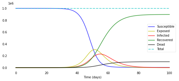
Note that I added a “total” that adds up S, E, I, R, and D for every time step as a “sanity check”: The compartments always have to sum up to N; this can give you a hint as to whether your equations are correct.
Time-Dependent Variables
Here’s an updated list of the variables we currently use:
- N: total population
- S(t): number of people susceptible on day t
- E(t): number of people exposed on day t
- I(t): number of people infected on day t
- R(t): number of people recovered on day t
- D(t): number of people dead on day t
- $\beta$: expected amount of people an infected person infects per day
- D: number of days an infected person has and can spread the disease
- $\gamma$: the proportion of infected recovering per day ($\gamma$ = 1/D)
- $R_0$: the total number of people an infected person infects ($R_0 = \beta / \gamma$)
- $\delta$: length of incubation period
- $\alpha$: fatality rate
- $\rho$: rate at which people die (= 1/days from infected until death)
As you can see, only the compartments change over time (they are not constant). Ofcourse, this is highly unrealistic! As an example, $R_0$ is usually not a constant because nationwide lockdowns reduce the number of people an infected person infects. Naturally, to get closer to modelling real-world developments, we have to make our variables change over time.
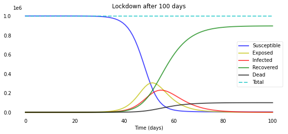
Time-Dependent $R_0$
First, we implement a simple change: on day L, a strict “lockdown” is enforced, pushing $R_0$ to 0.9. In the equations, we use β and not R₀, but we know that $R_0 = \beta / \gamma$, so $\beta = R_0 ⋅ \gamma$. That means that we define the following function:
L = 100
N = 1000000
D = 4.0 # infections lasts four days
gamma = 1.0 / D
delta = 1.0 / 5.0  # incubation period of five days

def R_0(t):
    return 5 if t < L else 0.9

def deriv(y, t, N, beta, gamma, delta, alpha, rho):
    S, E, I, R, D = y
    dSdt = -beta(t) * S * I / N
    dEdt = beta(t) * S * I / N - delta * E
    dIdt = delta * E - (1 - alpha) * gamma * I - alpha * rho * I
    dRdt = (1 - alpha) * gamma * I
    dDdt = alpha * rho * I
    return dSdt, dEdt, dIdt, dRdt, dDdt
and another function for beta that calls this function:
def beta(t):
    return R_0(t) * gamma

alpha = 0.2  # 10% death rate
rho = 1/9  # 9 days from infection until death
S0, E0, I0, R0, D0 = N-1, 1, 0, 0, 0  # initial conditions: one exposed
t = np.linspace(0, 100, 100) # Grid of time points (in days)
y0 = S0, E0, I0, R0, D0 # Initial conditions vector

# Integrate the SIR equations over the time grid, t.
ret = odeint(deriv, y0, t, args=(N, beta, gamma, delta, alpha, rho))
S, E, I, R, D = ret.T

plotsir(t, S, E, I, R, D, L)
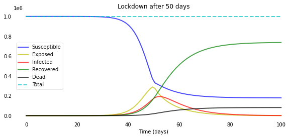
Let’s plot this for some different values of L:
L = 50
N = 1_000_000
D = 4.0 # infections lasts four days
gamma = 1.0 / D
delta = 1.0 / 5.0  # incubation period of five days

alpha = 0.2  # 10% death rate
rho = 1/9  # 9 days from infection until death
S0, E0, I0, R0, D0 = N-1, 1, 0, 0, 0  # initial conditions: one exposed

t = np.linspace(0, 100, 100) # Grid of time points (in days)
y0 = S0, E0, I0, R0, D0 # Initial conditions vector

# Integrate the SIR equations over the time grid, t.
ret = odeint(deriv, y0, t, args=(N, beta, gamma, delta, alpha, rho))
S, E, I, R, D = ret.T

plotsir(t, S, E, I, R, D, L)
L = 40
N = 1_000_000
D = 4.0 # infections lasts four days
gamma = 1.0 / D
delta = 1.0 / 5.0  # incubation period of five days

def R_0(t):
    return 5 if t < L else 0.9

def beta(t):
    return R_0(t) * gamma       # R_0 = beta / gamma, so beta = R_0 * gamma

alpha = 0.2  # 10% death rate
rho = 1/9  # 9 days from infection until death
S0, E0, I0, R0, D0 = N-1, 1, 0, 0, 0  # initial conditions: one exposed

t = np.linspace(0, 100, 100) # Grid of time points (in days)
y0 = S0, E0, I0, R0, D0 # Initial conditions vector

# Integrate the SIR equations over the time grid, t.
ret = odeint(deriv, y0, t, args=(N, beta, gamma, delta, alpha, rho))
S, E, I, R, D = ret.T

plotsir(t, S, E, I, R, D, L)
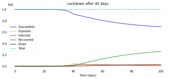
A few days can make a huge difference in the overall spread of the disease!
In reality, $R_0$ probably never “jumps” from one value to another. Rather, it (more or less quickly) continuously changes (and might go up and down several times, e.g. if social distancing measures are loosened and then tightened again). You can choose any function you want for $R_0$, one common choice to model the initial impact of social distancing: a logistic function.
The function (adopted for our purposes) looks like this:
And here’s what the parameters actually do:
- $R_0$start and $R_0$end are the values of $R_0$ on the first and the last day
- $x_0$ is the x-value of the inflection point (i.e. the date of the steepest decline in $R_0$, this could be thought of as the main “lockdown” date)
- k lets us vary how quickly $R_0$ declines
Again, changing the code accordingly:
def plotseird(t, S, E, I, R, D=None, L=None, R0=None, Alpha=None, CFR=None):
    f, ax = plt.subplots(1,1,figsize=(10,4))
    ax.plot(t, S, 'b', alpha=0.7, linewidth=2, label='Susceptible')
    ax.plot(t, E, 'y', alpha=0.7, linewidth=2, label='Exposed')
    ax.plot(t, I, 'r', alpha=0.7, linewidth=2, label='Infected')
    ax.plot(t, R, 'g', alpha=0.7, linewidth=2, label='Recovered')
    if D is not None:
        ax.plot(t, D, 'k', alpha=0.7, linewidth=2, label='Dead')
        ax.plot(t, S+E+I+R+D, 'c--', alpha=0.7, linewidth=2, label='Total')
    else:
        ax.plot(t, S+E+I+R, 'c--', alpha=0.7, linewidth=2, label='Total')

    ax.set_xlabel('Time (days)')

    ax.yaxis.set_tick_params(length=0)
    ax.xaxis.set_tick_params(length=0)
    ax.grid(b=True, which='major', c='w', lw=2, ls='-')
    legend = ax.legend(borderpad=2.0)
    legend.get_frame().set_alpha(0.5)
    for spine in ('top', 'right', 'bottom', 'left'):
        ax.spines[spine].set_visible(False)
    if L is not None:
        plt.title("Lockdown after {} days".format(L))
    plt.show();

    if R0 is not None or CFR is not None:
        f = plt.figure(figsize=(12,4))

    if R0 is not None:
    # sp1
        ax1 = f.add_subplot(121)
        ax1.plot(t, R0, 'b--', alpha=0.7, linewidth=2, label='R_0')

        ax1.set_xlabel('Time (days)')
        ax1.title.set_text('R_0 over time')
    # ax.set_ylabel('Number (1000s)')
    # ax.set_ylim(0,1.2)
        ax1.yaxis.set_tick_params(length=0)
        ax1.xaxis.set_tick_params(length=0)
        ax1.grid(b=True, which='major', c='w', lw=2, ls='-')
        legend = ax1.legend()
        legend.get_frame().set_alpha(0.5)
        for spine in ('top', 'right', 'bottom', 'left'):
              ax.spines[spine].set_visible(False)

    if Alpha is not None:
    # sp2
        ax2 = f.add_subplot(122)
        ax2.plot(t, Alpha, 'r--', alpha=0.7, linewidth=2, label='alpha')

        ax2.set_xlabel('Time (days)')
        ax2.title.set_text('fatality rate over time')
    # ax.set_ylabel('Number (1000s)')
    # ax.set_ylim(0,1.2)
        ax2.yaxis.set_tick_params(length=0)
        ax2.xaxis.set_tick_params(length=0)
        ax2.grid(b=True, which='major', c='w', lw=2, ls='-')
        legend = ax2.legend()
        legend.get_frame().set_alpha(0.5)
        for spine in ('top', 'right', 'bottom', 'left'):
            ax.spines[spine].set_visible(False)

    plt.show();
def deriv(y, t, N, beta, gamma, delta, alpha, rho):
S, E, I, R, D = y
dSdt = -beta(t) * S * I / N
dEdt = beta(t) * S * I / N - delta * E
dIdt = delta * E - (1 - alpha) * gamma * I - alpha * rho * I
dRdt = (1 - alpha) * gamma * I
dDdt = alpha * rho * I
return dSdt, dEdt, dIdt, dRdt, dDdt
N = 1_000_000
D = 4.0 # infections lasts four days
gamma = 1.0 / D
delta = 1.0 / 5.0 # incubation period of five days
R_0_start, k, x0, R_0_end = 5.0, 0.5, 50, 0.5
def logistic_R_0(t):
return (R_0_start-R_0_end) / (1 + np.exp(-k*(-t+x0))) + R_0_end
def beta(t):
return logistic_R_0(t) * gamma
alpha = 0.2 # 20% death rate
rho = 1/9 # 9 days from infection until death
S0, E0, I0, R0, D0 = N-1, 1, 0, 0, 0 # initial conditions: one exposed
t = np.linspace(0, 100, 100) # Grid of time points (in days)
y0 = S0, E0, I0, R0, D0 # Initial conditions vector
# Integrate the SIR equations over the time grid, t.
ret = odeint(deriv, y0, t, args=(N, beta, gamma, delta, alpha, rho))
S, E, I, R, D = ret.T
R0_over_time = [logistic_R_0(i) for i in range(len(t))] # to plot R_0 over time: get function values
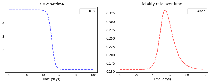
plotseird(t, S, E, I, R, D, R0=R0_over_time)
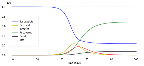
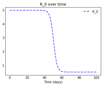
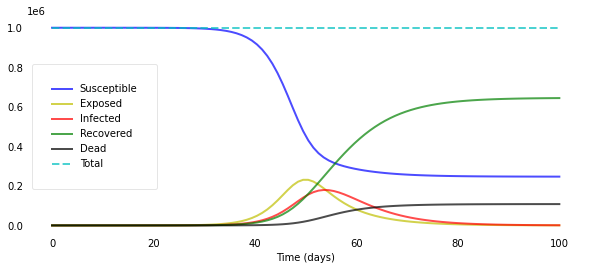
We let $R_0$ decline quickly from 5.0 to 0.5 around day 50 and can now really see the curves flattening after day 50.
Resource- and Age-Dependent Fatality Rates
Similarly to $R_0$, the fatality rate $\alpha$ is probably not constant for most real diseases. It might depend on a variety of things; We’ll focus on dependency on resources and age.
First, let’s look at resource dependency. We want the fatality rate to be higher when more people are infected. Think about how this could be put into a function: we probably need a “base” or “optimal” fatality rate for the case that only few people are infected (and thus receive optimal treatment) and some factor that takes into account what proportion of the population is currently infected. This is one example of a function that implements these ideas:
Here, s is some arbitrary but fixed scaling factor that controls how big of an influence the proportion of infected should have. For example, if s=1 and half the population is infected on one day, then s ⋅ I(t) / N = 1⁄2, so the fatality rate on that day is 50% + $\alpha_{OPT}$. Or maybe most people barely have any symptoms and thus many people being infected does not clog the hospitals.
Age dependency is a little more difficult. To fully implement it, we’d have to include separate compartments for every age group (e.g. an Infected-compartment for people aged 0–9, another one for people aged 10–19, …). That’s doable with a simple for-loop in python, but the equations get a little messy. A simpler approach that still is able to produce good results is the following:
We need 2 things for the simpler approach: Fatality rates by age group and proportion of the total population that is in that age group. For example, we might have the following fatality rates and number of individuals by age group (in Python dictionaries):
alpha_by_agegroup = {"0-29": 0.01, "30-59": 0.05, "60-89": 0.2, "89+": 0.3}
proportion_of_agegroup = {"0-29": 0.1, "30-59": 0.3, "60-89": 0.4, "89+": 0.2}
(This would be an extremely old population with 40% being in the 60–89 range and 20% being in the 89+ range). Now we calculate the overall average fatality rate by adding up the age group fatality rate multiplied with the proportion of the population in that age group:
$\alpha$ = 0.01 ⋅ 0.1 + 0.05 ⋅ 0.3 + 0.2 ⋅ 0.4 + 0.3 ⋅ 0.2 = 15.6%.
alpha_opt = sum(alpha_by_agegroup[i] * proportion_of_agegroup[i] for i in list(alpha_by_agegroup.keys()))
If we want to use both our formulas for resource- and age-dependency, we could use the resource-formula we just used to calculate $\alpha_{OPT}$ and use that in our resource-dependent formula from above.
There are certainly more elaborate ways to implement fatality rates over time. For example, we’re not taking into account that only critical cases needing intensive care fill up the hospitals and might increase fatality rates; or that deaths change the population structure that we used to calculate the fatality rate in the first place; or that the impact of infected on fatality rates should take place several days later as people don’t usually die immediately, which would result in a Delay Differential Equation, and that’s annoying to deal with in Python!
Implementing Resource- and Age-Dependent Fatality Rates
This is rather straightforward, we don’t even have to change our main equations (we define alpha inside the equations as we need access to the current value I(t)).
With the fatality rates by age group and the older population from above (and a scaling factor s of 1, so many people being infected has a high impact on fatality rates)
def deriv(y, t, N, beta, gamma, delta, alpha_opt, rho):
    S, E, I, R, D = y

    def alpha(t):
        return s * I/N + alpha_opt
    dSdt = -beta(t) * S * I/N
    dEdt = beta(t) * S * I/N - delta * E
    dIdt = delta * E - (1 - alpha(t)) * gamma * I - alpha(t) * rho * I
    dRdt = (1 - alpha(t)) * gamma * I
    dDdt = alpha(t) * rho * I
    return dSdt, dEdt, dIdt, dRdt, dDdt

N = 1_000_000
D = 4.0 # infections last four days
gamma = 1.0 / D
delta = 1.0/5.0 # incubation period of five days

R_0_start, k, x0, R_0_end = 5.0, 0.5, 50, 0.5

s = 1.0

def logistic_R_0(t):
    return (R_0_start-R_0_end) / (1 + np.exp(-k*(-t+x0))) + R_0_end

def beta(t):
    return logistic_R_0(t) * gamma

rho = 1/9  # 9 days from infection until death
S0, E0, I0, R0, D0 = N-1, 1, 0, 0, 0  # initial conditions: one exposed

t = np.linspace(0, 100, 100) # Grid of time points (in days)
y0 = S0, E0, I0, R0, D0 # Initial conditions vector

# Integrate the SIR equations over the time grid, t.
ret = odeint(deriv, y0, t, args=(N, beta, gamma, delta, alpha_opt, rho))
S, E, I, R, D = ret.T

R0_over_time = [logistic_R_0(i) for i in range(len(t))]  # to plot R_0 over time: get function values

Alpha_over_time = [s * I[i]/N + alpha_opt for i in range(len(t))]  # to plot alpha over time
We arrive at this plot:
plotseird(t, S, E, I, R, D, R0=R0_over_time, Alpha=Alpha_over_time)