The objective of this project is to minimize wastage of meal kits in retail stores. Currently, this is being done by tracking each individual item from the source until the point of sale. This is a cumbersome process and is labor intensive. In order to realize the objective using machine learning the first step in the process is to have an accurate forecast of the demand. This project focuses on generating accurate forecast for each individual item (46 unique items) for each store (47 unique stores). There are three datasets that have been used for demand forecasting.
- Product dataset
- Product_ID
- Cook Products
- Sales Product
- ShelfLife_after_Cook
- ShelfLife_WFM
- Price
- Cost
- Product_ID
Locations dataset
- Cook_Loc
- Sales_Loc
- Market
- Cook_Loc
Sales dataset
- Locationno
- Market
- Saledate
- Productid
- Unit_gross_sales
- Locationno
Note: The unaltered dataset is not shared. Locations dataset contains features obtained from https://censusreporter.org/ not present in the original dataset
# import necessary libraries
import numpy as np
import pandas as pd
import matplotlib.pyplot as plt # visualization
import seaborn as sns  # visualization
import holidays   # stored list of holidays in U.S.

# Model
import lightgbm as lgb
import shap                  # For error analysis
from sklearn.model_selection import TimeSeriesSplit, GridSearchCV, RandomizedSearchCV
from sklearn.metrics import make_scorer
from sklearn.preprocessing import LabelEncoder

# Configuration
import warnings
warnings.filterwarnings('ignore')
pd.set_option('display.max_columns', None)
pd.set_option('display.max_rows', None)
# Read the dataset containing the products and sales of the products across the stores in the state of Texas

prod = pd.read_csv('WFM_Products', delimiter = '\t')
locations = pd.read_csv("locations.csv")
sales = pd.read_csv('WFM_Sales.txt', delimiter = '\t',  usecols = ['LOCATIONNO', 'MARKET', 'SALEDATE',
        'PRODUCTID', 'UNIT_GROSS_SALES'],
                    parse_dates = ['SALEDATE'])
Data Cleaning
Product dataset contains 9 missing values in the cost column. Client provided information for 4 of the nine missing values. Rest of the products were third party products thus were deemed unnecessary for the analysis. The price column contains ‘$’ symbol which was replaced and converted from string to float.
prod.isna().sum()
Product_ID              0
Cook Products           0
Sales Product           0
ShelfLife_after_Cook    0
ShelfLife_WFM           0
Price                   0
Cost                    9
dtype: int64
miss = {900979: 2.37, 901974: 1.78, 902588: 2.66,
902901: 2.15 }

for key, val in miss.items():
    for i in prod['Product_ID']:
#         print(i)
        if i == key:
            prod.at[prod[prod['Product_ID'] == i].index[0],'Cost'] = val


prod.dropna(inplace = True)
i = prod[prod['Product_ID']== 902901].index
prod.drop(i, inplace = True)
prod['Price'] = prod['Price'].str.replace('$', '').astype(float)
The third party items were removed from the sales column as well.
sales['Cost'] = sales['PRODUCTID'].map(prod.set_index('Product_ID')['Cost'])
index_names = sales[(sales['PRODUCTID'] == 902729) | (sales['PRODUCTID'] == 902322) | (sales['PRODUCTID'] == 902787) |
                   (sales['PRODUCTID'] == 902901) | (sales['PRODUCTID'] == 902323) | (sales['PRODUCTID'] == 902733) |
                   (sales['PRODUCTID'] == 902730) | (sales['PRODUCTID'] == 902732) | (sales['PRODUCTID'] == 902911) |
                    (sales['PRODUCTID'] == 901902) | (sales['PRODUCTID'] == 902547) | (sales['PRODUCTID'] == 902546)].index

sales.drop(index_names, inplace = True)
sales.dropna(inplace = True)
print(sales.shape, "\n")
sales.head()
(290014, 6)
| LOCATIONNO | MARKET | SALEDATE | PRODUCTID | UNIT_GROSS_SALES | Cost | |
|---|---|---|---|---|---|---|
| 1 | 10073 | Austin | 2019-09-08 | 902287 | 1.0 | 1.82 |
| 2 | 10086 | Austin | 2019-09-08 | 901352 | 1.0 | 2.28 |
| 4 | 10017 | Austin | 2019-09-08 | 901352 | 1.0 | 2.28 |
| 5 | 10085 | Austin | 2019-09-08 | 902714 | 1.0 | 1.96 |
| 6 | 10073 | Austin | 2019-09-08 | 902934 | 1.0 | 0.96 |
We check the total number of stores and number of unique items in the data. We also check the time range of the data.
# How many stores and items are there?
print("number of unique items :",sales.PRODUCTID.nunique())
print("number of unique store :",sales.LOCATIONNO.nunique())
number of unique items : 46
number of unique store : 47
# Time Range
sales["SALEDATE"].min(), sales["SALEDATE"].max()
(Timestamp('2019-09-08 00:00:00'), Timestamp('2021-04-06 00:00:00'))
Although, there are several unique items not all items are sold in all the stores. Most of the stores sell one less product except for store number 4, which sells ten less products. Each item and store is encoded using label encoder so that the store and item data can be incorporated in the model.
# How many items are in the store?
le = LabelEncoder()
sales['LOCATIONNO'] = le.fit_transform(sales['LOCATIONNO'].values)
inverse_loc = le.inverse_transform(sales['LOCATIONNO'])
trans_loc = sales['LOCATIONNO']
sales['PRODUCTID'] = le.fit_transform(sales['PRODUCTID'].values)
sales.groupby(["LOCATIONNO"])["PRODUCTID"].nunique()
LOCATIONNO
0     46
1     46
2     46
3     46
4     36
5     45
6     45
7     46
8     46
9     45
10    46
11    46
12    46
13    45
14    46
15    45
16    45
17    46
18    46
19    46
20    46
21    46
22    46
23    46
24    46
25    46
26    46
27    45
28    46
29    46
30    46
31    45
32    46
33    46
34    46
35    45
36    46
37    45
38    46
39    46
40    46
41    46
42    45
43    46
44    46
45    46
46    45
Name: PRODUCTID, dtype: int64
The next step is to look at the summary statistic for each store to find out which of the items is more popular. We also do the same for the stores. We find out that store number 1 outsells most other stores.
# Summary Stats for each store
sales.groupby(["LOCATIONNO"]).agg({"UNIT_GROSS_SALES": ["count","sum", "mean",
                                                        "median", "std", "min", "max"]})
| UNIT_GROSS_SALES | |||||||
|---|---|---|---|---|---|---|---|
| count | sum | mean | median | std | min | max | |
| LOCATIONNO | |||||||
| 0 | 7466 | 22435.23 | 3.004987 | 2.0 | 2.688379 | 0.0 | 25.0 |
| 1 | 6624 | 15233.00 | 2.299668 | 2.0 | 1.962819 | 0.0 | 14.0 |
| 2 | 7430 | 18278.17 | 2.460050 | 2.0 | 2.107790 | 0.0 | 16.0 |
| 3 | 6367 | 11731.00 | 1.842469 | 1.0 | 1.621748 | 0.0 | 14.0 |
| 4 | 4890 | 17768.00 | 3.633538 | 3.0 | 3.411545 | 0.0 | 36.0 |
| 5 | 5095 | 8027.75 | 1.575613 | 1.0 | 1.507925 | 0.0 | 13.0 |
| 6 | 5224 | 8745.00 | 1.674005 | 1.0 | 1.619680 | 0.0 | 14.0 |
| 7 | 5487 | 9790.80 | 1.784363 | 1.0 | 1.819337 | 0.0 | 20.0 |
| 8 | 5358 | 10026.00 | 1.871221 | 1.0 | 1.705230 | 0.0 | 12.0 |
| 9 | 5097 | 6627.00 | 1.300177 | 1.0 | 1.319514 | 0.0 | 9.0 |
| 10 | 4956 | 7925.70 | 1.599213 | 1.0 | 1.520835 | 0.0 | 11.0 |
| 11 | 4520 | 5239.00 | 1.159071 | 1.0 | 1.248378 | 0.0 | 10.0 |
| 12 | 6262 | 19845.88 | 3.169256 | 2.0 | 2.914780 | 0.0 | 30.0 |
| 13 | 4651 | 5736.00 | 1.233283 | 1.0 | 1.275230 | 0.0 | 12.0 |
| 14 | 5726 | 13203.00 | 2.305798 | 2.0 | 2.081381 | 0.0 | 16.0 |
| 15 | 5738 | 12329.29 | 2.148709 | 2.0 | 2.003545 | 0.0 | 16.1 |
| 16 | 5379 | 9544.90 | 1.774475 | 1.0 | 1.721056 | 0.0 | 18.0 |
| 17 | 6903 | 16933.00 | 2.452991 | 2.0 | 2.094687 | 0.0 | 16.0 |
| 18 | 6389 | 12324.00 | 1.928940 | 2.0 | 1.671323 | 0.0 | 20.0 |
| 19 | 7158 | 17659.00 | 2.467030 | 2.0 | 2.074877 | 0.0 | 15.0 |
| 20 | 6254 | 10149.00 | 1.622801 | 1.0 | 1.457495 | 0.0 | 12.0 |
| 21 | 6634 | 12702.00 | 1.914682 | 2.0 | 1.650885 | 0.0 | 13.0 |
| 22 | 6617 | 10787.00 | 1.630195 | 1.0 | 1.533882 | 0.0 | 15.0 |
| 23 | 6887 | 12882.00 | 1.870481 | 2.0 | 1.617796 | 0.0 | 14.0 |
| 24 | 6988 | 17344.00 | 2.481969 | 2.0 | 2.162589 | 0.0 | 18.0 |
| 25 | 6381 | 11172.00 | 1.750823 | 1.0 | 1.573079 | 0.0 | 16.0 |
| 26 | 6736 | 14235.00 | 2.113272 | 2.0 | 1.740413 | 0.0 | 12.0 |
| 27 | 6319 | 13571.00 | 2.147650 | 2.0 | 2.002659 | 0.0 | 16.0 |
| 28 | 6318 | 10464.00 | 1.656220 | 1.0 | 1.418869 | 0.0 | 11.0 |
| 29 | 5911 | 9410.42 | 1.592018 | 1.0 | 1.396673 | 0.0 | 15.0 |
| 30 | 8480 | 49427.82 | 5.828752 | 4.0 | 5.271472 | 0.0 | 85.0 |
| 31 | 5992 | 8855.00 | 1.477804 | 1.0 | 1.367350 | 0.0 | 18.0 |
| 32 | 7301 | 17564.35 | 2.405746 | 2.0 | 2.044244 | 0.0 | 25.0 |
| 33 | 7849 | 24421.02 | 3.111354 | 3.0 | 2.600314 | 0.0 | 22.0 |
| 34 | 5941 | 7162.00 | 1.205521 | 1.0 | 1.216750 | 0.0 | 11.0 |
| 35 | 5561 | 8248.25 | 1.483231 | 1.0 | 1.373421 | 0.0 | 12.0 |
| 36 | 5699 | 11326.00 | 1.987366 | 1.0 | 2.049454 | 0.0 | 29.0 |
| 37 | 5653 | 7343.00 | 1.298956 | 1.0 | 1.254628 | 0.0 | 9.0 |
| 38 | 6153 | 11187.00 | 1.818137 | 1.0 | 1.590339 | 0.0 | 13.0 |
| 39 | 6677 | 15645.00 | 2.343118 | 2.0 | 2.166764 | 0.0 | 22.0 |
| 40 | 6492 | 11928.00 | 1.837338 | 2.0 | 1.541209 | 0.0 | 14.0 |
| 41 | 6305 | 11331.00 | 1.797145 | 1.0 | 1.547141 | 0.0 | 12.0 |
| 42 | 6215 | 13815.00 | 2.222848 | 2.0 | 2.045364 | 0.0 | 15.0 |
| 43 | 5702 | 7844.00 | 1.375658 | 1.0 | 1.373397 | 0.0 | 12.0 |
| 44 | 6511 | 12741.73 | 1.956954 | 2.0 | 1.667920 | 0.0 | 18.0 |
| 45 | 6309 | 10392.00 | 1.647171 | 1.0 | 1.557735 | 0.0 | 13.0 |
| 46 | 5409 | 7842.00 | 1.449806 | 1.0 | 1.300789 | 0.0 | 12.0 |
# Summary Stats for each item
sales.groupby(["PRODUCTID"]).agg({"UNIT_GROSS_SALES": ["count","sum", "mean", "median",
                                                       "std", "min", "max"]})
| UNIT_GROSS_SALES | |||||||
|---|---|---|---|---|---|---|---|
| count | sum | mean | median | std | min | max | |
| PRODUCTID | |||||||
| 0 | 881 | 1489.00 | 1.690125 | 1.0 | 1.149310 | 1.00 | 12.0 |
| 1 | 15271 | 39342.84 | 2.576311 | 2.0 | 2.507954 | 0.00 | 28.0 |
| 2 | 8558 | 23905.00 | 2.793293 | 2.0 | 2.145337 | 0.00 | 22.0 |
| 3 | 18194 | 51367.75 | 2.823335 | 2.0 | 2.821902 | 0.00 | 59.0 |
| 4 | 100 | 165.00 | 1.650000 | 1.0 | 1.192358 | 1.00 | 7.0 |
| 5 | 6961 | 15097.77 | 2.168908 | 2.0 | 1.496724 | 0.42 | 16.0 |
| 6 | 5752 | 13468.00 | 2.341446 | 2.0 | 1.631576 | 0.00 | 13.0 |
| 7 | 3199 | 5679.00 | 1.775242 | 1.0 | 1.152993 | 0.00 | 13.0 |
| 8 | 8967 | 21627.71 | 2.411923 | 2.0 | 2.707817 | 0.00 | 27.0 |
| 9 | 4387 | 7152.65 | 1.630419 | 1.0 | 0.942318 | 0.00 | 7.0 |
| 10 | 1002 | 1627.00 | 1.623752 | 1.0 | 1.042146 | 1.00 | 9.0 |
| 11 | 8836 | 12853.00 | 1.454617 | 0.0 | 2.310401 | 0.00 | 25.0 |
| 12 | 3086 | 5614.00 | 1.819183 | 1.0 | 1.048439 | 1.00 | 7.0 |
| 13 | 8958 | 17678.39 | 1.973475 | 1.0 | 2.339349 | 0.00 | 27.0 |
| 14 | 843 | 1317.00 | 1.562278 | 1.0 | 0.915348 | 1.00 | 7.0 |
| 15 | 6124 | 14881.00 | 2.429948 | 2.0 | 1.885544 | 0.00 | 22.0 |
| 16 | 11353 | 30249.00 | 2.664406 | 2.0 | 1.953958 | 0.00 | 25.0 |
| 17 | 4306 | 9994.81 | 2.321136 | 2.0 | 1.703804 | 0.11 | 15.0 |
| 18 | 2591 | 5086.00 | 1.962949 | 2.0 | 1.313200 | 1.00 | 11.0 |
| 19 | 1987 | 5283.00 | 2.658782 | 2.0 | 2.037989 | 0.00 | 18.0 |
| 20 | 5255 | 9629.00 | 1.832350 | 1.0 | 1.116143 | 1.00 | 11.0 |
| 21 | 1106 | 1902.50 | 1.720163 | 1.0 | 1.057462 | 1.00 | 8.5 |
| 22 | 6964 | 14536.00 | 2.087306 | 2.0 | 1.387399 | 0.00 | 14.0 |
| 23 | 2839 | 4561.00 | 1.606552 | 1.0 | 0.924477 | 0.00 | 11.0 |
| 24 | 3504 | 6131.00 | 1.749715 | 1.0 | 1.033758 | 1.00 | 8.0 |
| 25 | 5595 | 11575.00 | 2.068811 | 2.0 | 1.299769 | 0.00 | 10.0 |
| 26 | 3078 | 5623.00 | 1.826836 | 2.0 | 1.059599 | 0.00 | 9.0 |
| 27 | 13402 | 35149.25 | 2.622687 | 2.0 | 2.708546 | 0.00 | 35.0 |
| 28 | 4546 | 10005.00 | 2.200836 | 2.0 | 1.461169 | 0.00 | 14.0 |
| 29 | 3925 | 7301.00 | 1.860127 | 1.0 | 1.145417 | 1.00 | 8.0 |
| 30 | 1498 | 3500.00 | 2.336449 | 2.0 | 1.517748 | 1.00 | 13.0 |
| 31 | 755 | 1435.00 | 1.900662 | 1.0 | 1.301677 | 0.00 | 9.0 |
| 32 | 1358 | 2502.00 | 1.842415 | 1.0 | 1.160730 | 0.00 | 11.0 |
| 33 | 6111 | 13937.90 | 2.280789 | 2.0 | 1.605280 | 0.00 | 19.0 |
| 34 | 13443 | 31241.59 | 2.324004 | 2.0 | 2.274236 | 0.00 | 26.0 |
| 35 | 5769 | 11913.00 | 2.065003 | 2.0 | 1.470268 | 0.00 | 15.0 |
| 36 | 836 | 1309.00 | 1.565789 | 1.0 | 0.973531 | 1.00 | 7.0 |
| 37 | 13299 | 30004.98 | 2.256183 | 2.0 | 2.299639 | 0.00 | 57.0 |
| 38 | 13522 | 33390.15 | 2.469320 | 2.0 | 2.412362 | 0.00 | 29.0 |
| 39 | 8837 | 9548.00 | 1.080457 | 0.0 | 1.863488 | 0.00 | 22.0 |
| 40 | 8836 | 10658.50 | 1.206258 | 0.0 | 1.859811 | 0.00 | 23.0 |
| 41 | 8836 | 18154.00 | 2.054550 | 1.0 | 3.142165 | 0.00 | 85.0 |
| 42 | 8836 | 19553.76 | 2.212965 | 1.0 | 3.178544 | 0.00 | 43.0 |
| 43 | 8836 | 13038.76 | 1.475641 | 0.0 | 2.216686 | 0.00 | 31.0 |
| 44 | 8836 | 9877.00 | 1.117813 | 0.0 | 1.928911 | 0.00 | 25.0 |
| 45 | 8836 | 8837.00 | 1.000113 | 0.0 | 1.571769 | 0.00 | 15.0 |
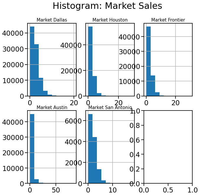
sns.set_context("talk", font_scale=1.4)
markets = ['Dallas', 'Houston', 'Frontier', 'Austin', 'San Antonio']

fig, axes = plt.subplots(2, 3, figsize=(10, 10))
for i in range(len(markets)):
    if i < 3:
        sales[sales.MARKET == markets[i]].UNIT_GROSS_SALES.hist(ax=axes[0, i])
        axes[0,i].set_title("Market " + markets[i], fontsize = 15)
    else:
        sales[sales.MARKET == markets[i]].UNIT_GROSS_SALES.hist(ax=axes[1, i-3])
        axes[1,i-3].set_title("Market " + markets[i], fontsize = 15)

plt.tight_layout(pad= 4.5)
plt.suptitle("Histogram: Market Sales");
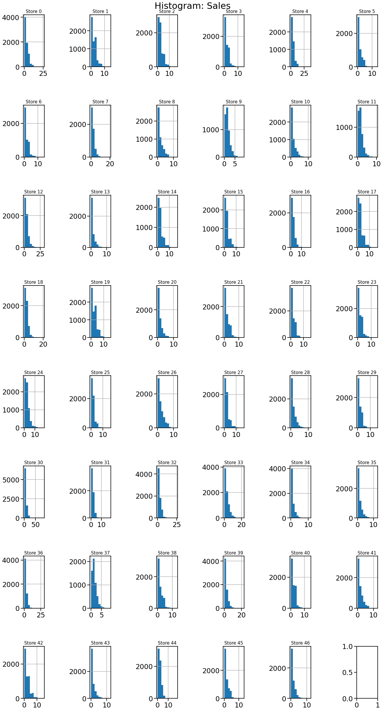
# Histogram Sales
sns.set_context("talk", font_scale=1.4)
fig, axes = plt.subplots(8, 6, figsize=(20, 35))
for i in range(0,47):
    if i < 6:
        sales[sales.LOCATIONNO == i].UNIT_GROSS_SALES.hist(ax=axes[0, i])
        axes[0,i].set_title("Store " + str(i), fontsize = 15)

    elif (i > 5) & (i < 12):
        sales[sales.LOCATIONNO == i].UNIT_GROSS_SALES.hist(ax=axes[1, i - 6])
        axes[1,i-6].set_title("Store " + str(i), fontsize = 15)

    elif (i > 11) & (i < 18):
        sales[sales.LOCATIONNO == i].UNIT_GROSS_SALES.hist(ax=axes[2, i - 12])
        axes[2,i-12].set_title("Store " + str(i), fontsize = 15)

    elif (i > 17) & (i < 24):
        sales[sales.LOCATIONNO == i].UNIT_GROSS_SALES.hist(ax=axes[3, i - 18])
        axes[3,i-18].set_title("Store " + str(i), fontsize = 15)

    elif (i > 23) & (i < 30):
        sales[sales.LOCATIONNO == i].UNIT_GROSS_SALES.hist(ax=axes[4, i - 24])
        axes[4,i-24].set_title("Store " + str(i), fontsize = 15)

    elif (i > 29) & (i < 36):
        sales[sales.LOCATIONNO == i].UNIT_GROSS_SALES.hist(ax=axes[5, i - 30])
        axes[5,i-30].set_title("Store " + str(i), fontsize = 15)

    elif (i > 35) & (i < 42):
        sales[sales.LOCATIONNO == i].UNIT_GROSS_SALES.hist(ax=axes[6, i - 36])
        axes[6,i-36].set_title("Store " + str(i), fontsize = 15)

    else:
        sales[sales.LOCATIONNO == i].UNIT_GROSS_SALES.hist(ax=axes[7, i - 42])
        axes[7,i-42].set_title("Store " + str(i), fontsize = 15)

plt.tight_layout(pad= 3)
plt.suptitle("Histogram: Sales");

The following plot shows the sale of all the items in store 1.
store = 1
sub = sales[sales.LOCATIONNO == store].set_index("SALEDATE")

# sns.set_context("talk", font_scale=1.4)
fig, axes = plt.subplots(8, 6, figsize=(35, 40))
for i in range(0,46):
    if i < 6:
        sub[sub.PRODUCTID == i].UNIT_GROSS_SALES.plot(ax=axes[0, i],
                                      legend=True, label = "Item "+str(i)+" Sales")
    elif (i > 5) & (i < 12):
        sub[sub.PRODUCTID == i].UNIT_GROSS_SALES.plot(ax=axes[1, i - 6],
                                      legend=True, label = "Item "+str(i)+" Sales")
    elif (i > 11) & (i < 18):
        sub[sub.PRODUCTID == i].UNIT_GROSS_SALES.plot(ax=axes[2, i - 12],
                                      legend=True, label = "Item "+str(i)+" Sales")
    elif (i > 17) & (i < 24):
        sub[sub.PRODUCTID == i].UNIT_GROSS_SALES.plot(ax=axes[3, i - 18],
                                      legend=True, label = "Item "+str(i)+" Sales")
    elif (i > 23) & (i < 30):
        sub[sub.PRODUCTID == i].UNIT_GROSS_SALES.plot(ax=axes[4, i - 24],
                                      legend=True, label = "Item "+str(i)+" Sales")
    elif (i > 29) & (i < 36):
        sub[sub.PRODUCTID == i].UNIT_GROSS_SALES.plot(ax=axes[5, i - 30],
                                      legend=True, label = "Item "+str(i)+" Sales")
    elif (i > 35) & (i < 42):
        sub[sub.PRODUCTID == i].UNIT_GROSS_SALES.plot(ax=axes[6, i - 36],
                                      legend=True, label = "Item "+str(i)+" Sales")
    else:
        sub[sub.PRODUCTID == i].UNIT_GROSS_SALES.plot(ax=axes[7, i - 42],
                                      legend=True, label = "Item "+str(i)+" Sales")

plt.tight_layout(pad=3)
plt.suptitle("Store 1 Items");
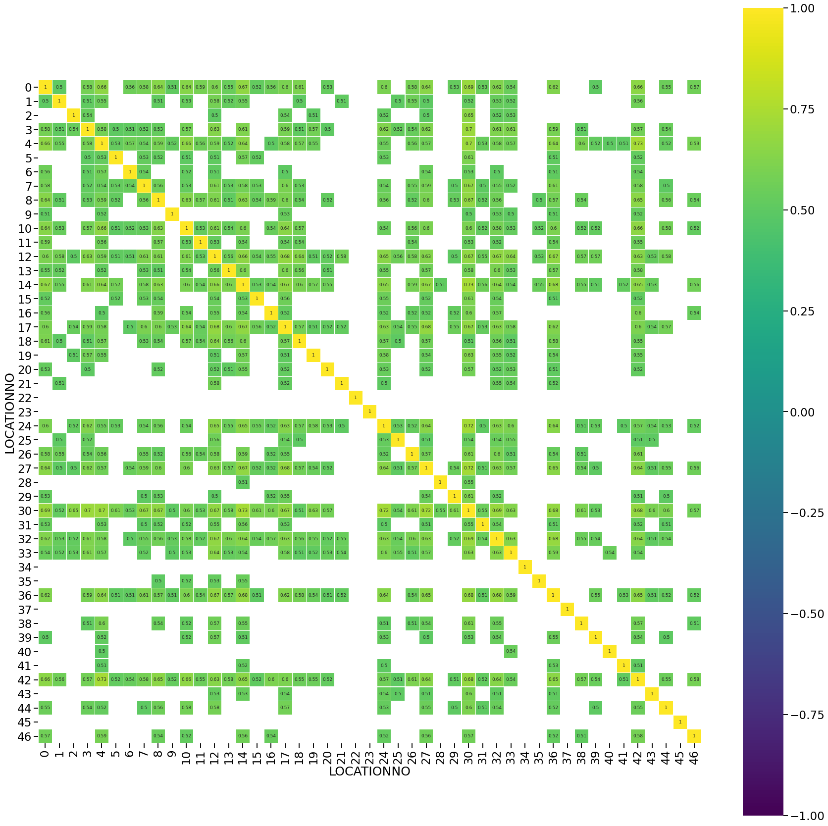
We check for correlation of total sales in each of the stores to find out if there stores or market that are correlated to one another. Based on the correlation data we can remove redundant data to improve the model prediction accuracy
# Correlation between total sales of stores

storesales = sales.groupby(["SALEDATE", "LOCATIONNO"]).UNIT_GROSS_SALES.sum().reset_index().set_index("SALEDATE")
corr =  pd.pivot_table(storesales, values = "UNIT_GROSS_SALES", columns="LOCATIONNO", index="SALEDATE").corr(method = "spearman")
plt.figure(figsize = (30,30))
sns.heatmap(corr[(corr >= 0.5) | (corr <= -0.5)],
            cmap='viridis', vmax=1.0, vmin=-1.0, linewidths=0.1,
            annot=True, annot_kws={"size": 9}, square=True);
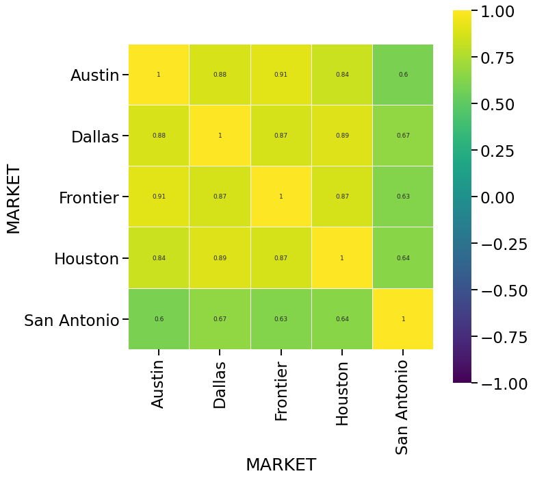
# Correlation between total sales at market level

sns.set_context("talk", font_scale=1.4)
marketsales = sales.groupby(["SALEDATE", "MARKET"]).UNIT_GROSS_SALES.sum().reset_index().set_index("SALEDATE")
corr =  pd.pivot_table(marketsales, values = "UNIT_GROSS_SALES", columns="MARKET", index="SALEDATE").corr(method = "spearman")
plt.figure(figsize = (10,10))
sns.heatmap(corr[(corr >= 0.5) | (corr <= -0.5)],
            cmap='viridis', vmax=1.0, vmin=-1.0, linewidths=0.1,
            annot=True, annot_kws={"size": 9}, square=True);
A non-parametric T-test is conducted to see which store sales are similar to each other. The same test is carried out for different items and different markets. This is incorporated during the feaure engineering phase of the project. This test is also called A/B testing.
# T Test
def CompareTwoGroups(dataframe, group, target):

    import itertools
    from scipy.stats import shapiro
    import scipy.stats as stats

    # 1. Normality Test: Shapiro Test
    # 2. Homogeneity Test: Levene Test
    # 3. Parametric or Non-Parametric T Test: T-Test, Welch Test, Mann Whitney U

    # Create Combinations
    item_comb = list(itertools.combinations(dataframe[group].unique(), 2))

    AB = pd.DataFrame()
    for i in range(0, len(item_comb)):
        # Define Groups
        groupA = dataframe[dataframe[group] == item_comb[i][0]][target]
        groupB = dataframe[dataframe[group] == item_comb[i][1]][target]

        # Assumption: Normality
        ntA = shapiro(groupA)[1] < 0.05
        ntB = shapiro(groupB)[1] < 0.05
        # H0: Distribution is Normal! - False
        # H1: Distribution is not Normal! - True

        if (ntA == False) & (ntB == False): # "H0: Normal Distribution"
            # Parametric Test
            # Assumption: Homogeneity of variances
            leveneTest = stats.levene(groupA, groupB)[1] < 0.05
            # H0: Homogeneity: False
            # H1: Heterogeneous: True
            if leveneTest == False:
                # Homogeneity
                ttest = stats.ttest_ind(groupA, groupB, equal_var=True)[1]
                # H0: M1 = M2 - False
                # H1: M1 != M2 - True
            else:
                # Heterogeneous
                ttest = stats.ttest_ind(groupA, groupB, equal_var=False)[1]
                # H0: M1 = M2 - False
                # H1: M1 != M2 - True
        else:
            # Non-Parametric Test
            ttest = stats.mannwhitneyu(groupA, groupB)[1]
            # H0: M1 = M2 - False
            # H1: M1 != M2 - True

        temp = pd.DataFrame({"Compare Two Groups":[ttest < 0.05],
                             "p-value":[ttest],
                             "GroupA_Mean":[groupA.mean()], "GroupB_Mean":[groupB.mean()],
                             "GroupA_Median":[groupA.median()], "GroupB_Median":[groupB.median()],
                             "GroupA_Count":[groupA.count()], "GroupB_Count":[groupB.count()]
                            }, index = [item_comb[i]])
        temp["Compare Two Groups"] = np.where(temp["Compare Two Groups"] == True, "Different Groups", "Similar Groups")
        temp["TestType"] = np.where((ntA == False) & (ntB == False), "Parametric", "Non-Parametric")

        AB = pd.concat([AB, temp[["TestType", "Compare Two Groups", "p-value","GroupA_Median", "GroupB_Median","GroupA_Mean", "GroupB_Mean",
                                 "GroupA_Count", "GroupB_Count"]]])

    return AB


ctg_store = CompareTwoGroups(storesales, group = "LOCATIONNO", target = "UNIT_GROSS_SALES")
ctg_ss = ctg_store[ctg_store["Compare Two Groups"] == "Similar Groups"]
ctg_ss
| TestType | Compare Two Groups | p-value | GroupA_Median | GroupB_Median | GroupA_Mean | GroupB_Mean | GroupA_Count | GroupB_Count | |
|---|---|---|---|---|---|---|---|---|---|
| (0, 2) | Non-Parametric | Similar Groups | 0.233386 | 31.0 | 32.0 | 38.950052 | 33.354325 | 576 | 548 |
| (20, 29) | Non-Parametric | Similar Groups | 0.337784 | 15.0 | 15.0 | 17.650435 | 17.266826 | 575 | 545 |
| (20, 36) | Non-Parametric | Similar Groups | 0.115768 | 15.0 | 15.0 | 17.650435 | 21.573333 | 575 | 525 |
| (20, 10) | Non-Parametric | Similar Groups | 0.472980 | 15.0 | 15.0 | 17.650435 | 18.136613 | 575 | 437 |
| (31, 35) | Non-Parametric | Similar Groups | 0.380683 | 14.0 | 14.0 | 15.453752 | 15.801245 | 573 | 522 |
| (31, 43) | Non-Parametric | Similar Groups | 0.310684 | 14.0 | 13.0 | 15.453752 | 14.912548 | 573 | 526 |
| (31, 46) | Non-Parametric | Similar Groups | 0.401160 | 14.0 | 13.0 | 15.453752 | 15.316406 | 573 | 512 |
| (31, 9) | Non-Parametric | Similar Groups | 0.361584 | 14.0 | 14.0 | 15.453752 | 14.959368 | 573 | 443 |
| (32, 17) | Non-Parametric | Similar Groups | 0.278548 | 27.5 | 27.0 | 30.599913 | 30.956124 | 574 | 547 |
| (32, 24) | Non-Parametric | Similar Groups | 0.281458 | 27.5 | 27.0 | 30.599913 | 31.649635 | 574 | 548 |
| (32, 14) | Non-Parametric | Similar Groups | 0.103080 | 27.5 | 26.0 | 30.599913 | 29.803612 | 574 | 443 |
| (33, 12) | Non-Parametric | Similar Groups | 0.275046 | 36.0 | 38.0 | 42.471339 | 44.900181 | 575 | 442 |
| (3, 22) | Non-Parametric | Similar Groups | 0.291572 | 18.0 | 19.0 | 21.446069 | 19.720293 | 547 | 547 |
| (3, 25) | Non-Parametric | Similar Groups | 0.388627 | 18.0 | 18.0 | 21.446069 | 20.424132 | 547 | 547 |
| (3, 28) | Non-Parametric | Similar Groups | 0.096847 | 18.0 | 17.0 | 21.446069 | 19.094891 | 547 | 548 |
| (3, 38) | Non-Parametric | Similar Groups | 0.059920 | 18.0 | 19.0 | 21.446069 | 21.227704 | 547 | 527 |
| (3, 45) | Non-Parametric | Similar Groups | 0.347969 | 18.0 | 18.0 | 21.446069 | 19.719165 | 547 | 527 |
| (3, 7) | Non-Parametric | Similar Groups | 0.208064 | 18.0 | 19.0 | 21.446069 | 22.051351 | 547 | 444 |
| (3, 16) | Non-Parametric | Similar Groups | 0.133355 | 18.0 | 19.0 | 21.446069 | 21.497523 | 547 | 444 |
| (17, 24) | Non-Parametric | Similar Groups | 0.146562 | 27.0 | 27.0 | 30.956124 | 31.649635 | 547 | 548 |
| (17, 39) | Non-Parametric | Similar Groups | 0.068823 | 27.0 | 25.0 | 30.956124 | 29.686907 | 547 | 527 |
| (17, 1) | Non-Parametric | Similar Groups | 0.142868 | 27.0 | 25.0 | 30.956124 | 29.070611 | 547 | 524 |
| (17, 14) | Non-Parametric | Similar Groups | 0.245477 | 27.0 | 26.0 | 30.956124 | 29.803612 | 547 | 443 |
| (18, 22) | Non-Parametric | Similar Groups | 0.078444 | 19.0 | 19.0 | 22.530165 | 19.720293 | 547 | 547 |
| (18, 27) | Non-Parametric | Similar Groups | 0.152819 | 19.0 | 20.0 | 22.530165 | 24.764599 | 547 | 548 |
| (18, 38) | Non-Parametric | Similar Groups | 0.389069 | 19.0 | 19.0 | 22.530165 | 21.227704 | 547 | 527 |
| (18, 41) | Non-Parametric | Similar Groups | 0.476575 | 19.0 | 20.0 | 22.530165 | 21.541825 | 547 | 526 |
| (18, 7) | Non-Parametric | Similar Groups | 0.216345 | 19.0 | 19.0 | 22.530165 | 22.051351 | 547 | 444 |
| (18, 16) | Non-Parametric | Similar Groups | 0.322617 | 19.0 | 19.0 | 22.530165 | 21.497523 | 547 | 444 |
| (18, 8) | Non-Parametric | Similar Groups | 0.407530 | 19.0 | 19.0 | 22.530165 | 22.734694 | 547 | 441 |
| (19, 24) | Non-Parametric | Similar Groups | 0.163828 | 29.0 | 27.0 | 32.224453 | 31.649635 | 548 | 548 |
| (21, 23) | Non-Parametric | Similar Groups | 0.160270 | 21.0 | 22.0 | 23.178832 | 23.507299 | 548 | 548 |
| (21, 27) | Non-Parametric | Similar Groups | 0.209002 | 21.0 | 20.0 | 23.178832 | 24.764599 | 548 | 548 |
| (21, 40) | Non-Parametric | Similar Groups | 0.471788 | 21.0 | 21.0 | 23.178832 | 22.633776 | 548 | 527 |
| (21, 42) | Non-Parametric | Similar Groups | 0.359416 | 21.0 | 20.0 | 23.178832 | 26.465517 | 548 | 522 |
| (21, 44) | Non-Parametric | Similar Groups | 0.213510 | 21.0 | 22.0 | 23.178832 | 24.177856 | 548 | 527 |
| (21, 8) | Non-Parametric | Similar Groups | 0.085189 | 21.0 | 19.0 | 23.178832 | 22.734694 | 548 | 441 |
| (22, 25) | Non-Parametric | Similar Groups | 0.187974 | 19.0 | 18.0 | 19.720293 | 20.424132 | 547 | 547 |
| (22, 38) | Non-Parametric | Similar Groups | 0.111677 | 19.0 | 19.0 | 19.720293 | 21.227704 | 547 | 527 |
| (22, 45) | Non-Parametric | Similar Groups | 0.179004 | 19.0 | 18.0 | 19.720293 | 19.719165 | 547 | 527 |
| (22, 7) | Non-Parametric | Similar Groups | 0.297087 | 19.0 | 19.0 | 19.720293 | 22.051351 | 547 | 444 |
| (22, 16) | Non-Parametric | Similar Groups | 0.141047 | 19.0 | 19.0 | 19.720293 | 21.497523 | 547 | 444 |
| (23, 40) | Non-Parametric | Similar Groups | 0.144820 | 22.0 | 21.0 | 23.507299 | 22.633776 | 548 | 527 |
| (23, 42) | Non-Parametric | Similar Groups | 0.284477 | 22.0 | 20.0 | 23.507299 | 26.465517 | 548 | 522 |
| (23, 44) | Non-Parametric | Similar Groups | 0.440538 | 22.0 | 22.0 | 23.507299 | 24.177856 | 548 | 527 |
| (25, 28) | Non-Parametric | Similar Groups | 0.141127 | 18.0 | 17.0 | 20.424132 | 19.094891 | 547 | 548 |
| (25, 45) | Non-Parametric | Similar Groups | 0.480488 | 18.0 | 18.0 | 20.424132 | 19.719165 | 547 | 527 |
| (25, 6) | Non-Parametric | Similar Groups | 0.062208 | 18.0 | 17.0 | 20.424132 | 19.740406 | 547 | 443 |
| (25, 7) | Non-Parametric | Similar Groups | 0.112849 | 18.0 | 19.0 | 20.424132 | 22.051351 | 547 | 444 |
| (25, 16) | Non-Parametric | Similar Groups | 0.057894 | 18.0 | 19.0 | 20.424132 | 21.497523 | 547 | 444 |
| (27, 38) | Non-Parametric | Similar Groups | 0.083419 | 20.0 | 19.0 | 24.764599 | 21.227704 | 548 | 527 |
| (27, 40) | Non-Parametric | Similar Groups | 0.218523 | 20.0 | 21.0 | 24.764599 | 22.633776 | 548 | 527 |
| (27, 41) | Non-Parametric | Similar Groups | 0.137742 | 20.0 | 20.0 | 24.764599 | 21.541825 | 548 | 526 |
| (27, 42) | Non-Parametric | Similar Groups | 0.146031 | 20.0 | 20.0 | 24.764599 | 26.465517 | 548 | 522 |
| (27, 44) | Non-Parametric | Similar Groups | 0.072787 | 20.0 | 22.0 | 24.764599 | 24.177856 | 548 | 527 |
| (27, 16) | Non-Parametric | Similar Groups | 0.068801 | 20.0 | 19.0 | 24.764599 | 21.497523 | 548 | 444 |
| (27, 8) | Non-Parametric | Similar Groups | 0.233037 | 20.0 | 19.0 | 24.764599 | 22.734694 | 548 | 441 |
| (28, 45) | Non-Parametric | Similar Groups | 0.157909 | 17.0 | 18.0 | 19.094891 | 19.719165 | 548 | 527 |
| (28, 5) | Non-Parametric | Similar Groups | 0.082682 | 17.0 | 17.0 | 19.094891 | 18.162330 | 548 | 442 |
| (28, 6) | Non-Parametric | Similar Groups | 0.282677 | 17.0 | 17.0 | 19.094891 | 19.740406 | 548 | 443 |
| (29, 36) | Non-Parametric | Similar Groups | 0.056004 | 15.0 | 15.0 | 17.266826 | 21.573333 | 545 | 525 |
| (29, 10) | Non-Parametric | Similar Groups | 0.340116 | 15.0 | 15.0 | 17.266826 | 18.136613 | 545 | 437 |
| (35, 43) | Non-Parametric | Similar Groups | 0.216217 | 14.0 | 13.0 | 15.801245 | 14.912548 | 522 | 526 |
| (35, 46) | Non-Parametric | Similar Groups | 0.272802 | 14.0 | 13.0 | 15.801245 | 15.316406 | 522 | 512 |
| (35, 9) | Non-Parametric | Similar Groups | 0.498473 | 14.0 | 14.0 | 15.801245 | 14.959368 | 522 | 443 |
| (37, 34) | Non-Parametric | Similar Groups | 0.478634 | 13.0 | 12.0 | 14.013359 | 13.615970 | 524 | 526 |
| (39, 1) | Non-Parametric | Similar Groups | 0.330655 | 25.0 | 25.0 | 29.686907 | 29.070611 | 527 | 524 |
| (39, 14) | Non-Parametric | Similar Groups | 0.232906 | 25.0 | 26.0 | 29.686907 | 29.803612 | 527 | 443 |
| (39, 15) | Non-Parametric | Similar Groups | 0.388649 | 25.0 | 26.0 | 29.686907 | 27.831354 | 527 | 443 |
| (1, 14) | Non-Parametric | Similar Groups | 0.364876 | 25.0 | 26.0 | 29.070611 | 29.803612 | 524 | 443 |
| (1, 15) | Non-Parametric | Similar Groups | 0.219119 | 25.0 | 26.0 | 29.070611 | 27.831354 | 524 | 443 |
| (36, 5) | Non-Parametric | Similar Groups | 0.323113 | 15.0 | 17.0 | 21.573333 | 18.162330 | 525 | 442 |
| (36, 6) | Non-Parametric | Similar Groups | 0.116215 | 15.0 | 17.0 | 21.573333 | 19.740406 | 525 | 443 |
| (36, 10) | Non-Parametric | Similar Groups | 0.125947 | 15.0 | 15.0 | 21.573333 | 18.136613 | 525 | 437 |
| (38, 41) | Non-Parametric | Similar Groups | 0.352019 | 19.0 | 20.0 | 21.227704 | 21.541825 | 527 | 526 |
| (38, 7) | Non-Parametric | Similar Groups | 0.304000 | 19.0 | 19.0 | 21.227704 | 22.051351 | 527 | 444 |
| (38, 16) | Non-Parametric | Similar Groups | 0.455081 | 19.0 | 19.0 | 21.227704 | 21.497523 | 527 | 444 |
| (38, 8) | Non-Parametric | Similar Groups | 0.247194 | 19.0 | 19.0 | 21.227704 | 22.734694 | 527 | 441 |
| (40, 42) | Non-Parametric | Similar Groups | 0.381842 | 21.0 | 20.0 | 22.633776 | 26.465517 | 527 | 522 |
| (40, 44) | Non-Parametric | Similar Groups | 0.188451 | 21.0 | 22.0 | 22.633776 | 24.177856 | 527 | 527 |
| (40, 8) | Non-Parametric | Similar Groups | 0.078163 | 21.0 | 19.0 | 22.633776 | 22.734694 | 527 | 441 |
| (41, 7) | Non-Parametric | Similar Groups | 0.204610 | 20.0 | 19.0 | 21.541825 | 22.051351 | 526 | 444 |
| (41, 16) | Non-Parametric | Similar Groups | 0.334767 | 20.0 | 19.0 | 21.541825 | 21.497523 | 526 | 444 |
| (41, 8) | Non-Parametric | Similar Groups | 0.338689 | 20.0 | 19.0 | 21.541825 | 22.734694 | 526 | 441 |
| (42, 44) | Non-Parametric | Similar Groups | 0.387730 | 20.0 | 22.0 | 26.465517 | 24.177856 | 522 | 527 |
| (43, 46) | Non-Parametric | Similar Groups | 0.432120 | 13.0 | 13.0 | 14.912548 | 15.316406 | 526 | 512 |
| (43, 9) | Non-Parametric | Similar Groups | 0.217890 | 13.0 | 14.0 | 14.912548 | 14.959368 | 526 | 443 |
| (45, 6) | Non-Parametric | Similar Groups | 0.072031 | 18.0 | 17.0 | 19.719165 | 19.740406 | 527 | 443 |
| (45, 7) | Non-Parametric | Similar Groups | 0.092305 | 18.0 | 19.0 | 19.719165 | 22.051351 | 527 | 444 |
| (46, 9) | Non-Parametric | Similar Groups | 0.298520 | 13.0 | 14.0 | 15.316406 | 14.959368 | 512 | 443 |
| (5, 6) | Non-Parametric | Similar Groups | 0.247393 | 17.0 | 17.0 | 18.162330 | 19.740406 | 442 | 443 |
| (5, 10) | Non-Parametric | Similar Groups | 0.062061 | 17.0 | 15.0 | 18.162330 | 18.136613 | 442 | 437 |
| (7, 16) | Non-Parametric | Similar Groups | 0.386442 | 19.0 | 19.0 | 22.051351 | 21.497523 | 444 | 444 |
| (7, 8) | Non-Parametric | Similar Groups | 0.151309 | 19.0 | 19.0 | 22.051351 | 22.734694 | 444 | 441 |
| (11, 13) | Non-Parametric | Similar Groups | 0.094553 | 10.0 | 11.0 | 12.071429 | 13.036364 | 434 | 440 |
| (14, 15) | Non-Parametric | Similar Groups | 0.134353 | 26.0 | 26.0 | 29.803612 | 27.831354 | 443 | 443 |
| (16, 8) | Non-Parametric | Similar Groups | 0.213394 | 19.0 | 19.0 | 21.497523 | 22.734694 | 444 | 441 |
itemsales = sales.groupby(["SALEDATE", "PRODUCTID"]).UNIT_GROSS_SALES.sum().reset_index().set_index("SALEDATE")
ctg_is = CompareTwoGroups(itemsales, group = "PRODUCTID", target = "UNIT_GROSS_SALES")
ctg_iss = ctg_is[ctg_is["Compare Two Groups"] == "Similar Groups"]
ctg_iss
| TestType | Compare Two Groups | p-value | GroupA_Median | GroupB_Median | GroupA_Mean | GroupB_Mean | GroupA_Count | GroupB_Count | |
|---|---|---|---|---|---|---|---|---|---|
| (6, 22) | Non-Parametric | Similar Groups | 0.431454 | 48.0 | 46.0 | 47.590106 | 49.274576 | 283 | 295 |
| (6, 25) | Non-Parametric | Similar Groups | 0.062028 | 48.0 | 46.0 | 47.590106 | 46.115538 | 283 | 251 |
| (6, 28) | Non-Parametric | Similar Groups | 0.191243 | 48.0 | 51.0 | 47.590106 | 49.776119 | 283 | 201 |
| (6, 18) | Non-Parametric | Similar Groups | 0.395740 | 48.0 | 47.0 | 47.590106 | 47.981132 | 283 | 106 |
| (6, 39) | Non-Parametric | Similar Groups | 0.282581 | 48.0 | 55.0 | 47.590106 | 50.518519 | 283 | 189 |
| (6, 44) | Non-Parametric | Similar Groups | 0.279319 | 48.0 | 57.0 | 47.590106 | 52.537234 | 283 | 188 |
| (6, 45) | Non-Parametric | Similar Groups | 0.437603 | 48.0 | 51.0 | 47.590106 | 47.005319 | 283 | 188 |
| (7, 32) | Non-Parametric | Similar Groups | 0.267717 | 24.5 | 20.0 | 25.581081 | 26.617021 | 222 | 94 |
| (7, 0) | Non-Parametric | Similar Groups | 0.110582 | 24.5 | 27.0 | 25.581081 | 26.589286 | 222 | 56 |
| (7, 10) | Non-Parametric | Similar Groups | 0.385214 | 24.5 | 26.0 | 25.581081 | 23.926471 | 222 | 68 |
| (7, 36) | Non-Parametric | Similar Groups | 0.234398 | 24.5 | 25.0 | 25.581081 | 22.964912 | 222 | 57 |
| (7, 14) | Non-Parametric | Similar Groups | 0.267800 | 24.5 | 24.0 | 25.581081 | 23.105263 | 222 | 57 |
| (9, 24) | Non-Parametric | Similar Groups | 0.061105 | 28.0 | 31.0 | 28.610600 | 30.809045 | 250 | 199 |
| (9, 21) | Non-Parametric | Similar Groups | 0.235222 | 28.0 | 32.0 | 28.610600 | 29.269231 | 250 | 65 |
| (9, 0) | Non-Parametric | Similar Groups | 0.292907 | 28.0 | 27.0 | 28.610600 | 26.589286 | 250 | 56 |
| (16, 19) | Non-Parametric | Similar Groups | 0.313315 | 78.0 | 79.0 | 78.568831 | 78.850746 | 385 | 67 |
| (16, 15) | Non-Parametric | Similar Groups | 0.106617 | 78.0 | 73.5 | 78.568831 | 77.505208 | 385 | 192 |
| (20, 29) | Non-Parametric | Similar Groups | 0.330028 | 33.0 | 34.0 | 34.389286 | 36.143564 | 280 | 202 |
| (20, 21) | Non-Parametric | Similar Groups | 0.066783 | 33.0 | 32.0 | 34.389286 | 29.269231 | 280 | 65 |
| (22, 25) | Non-Parametric | Similar Groups | 0.055195 | 46.0 | 46.0 | 49.274576 | 46.115538 | 295 | 251 |
| (22, 28) | Non-Parametric | Similar Groups | 0.271737 | 46.0 | 51.0 | 49.274576 | 49.776119 | 295 | 201 |
| (22, 18) | Non-Parametric | Similar Groups | 0.477400 | 46.0 | 47.0 | 49.274576 | 47.981132 | 295 | 106 |
| (22, 39) | Non-Parametric | Similar Groups | 0.377522 | 46.0 | 55.0 | 49.274576 | 50.518519 | 295 | 189 |
| (22, 44) | Non-Parametric | Similar Groups | 0.403045 | 46.0 | 57.0 | 49.274576 | 52.537234 | 295 | 188 |
| (22, 45) | Non-Parametric | Similar Groups | 0.413270 | 46.0 | 51.0 | 49.274576 | 47.005319 | 295 | 188 |
| (23, 30) | Non-Parametric | Similar Groups | 0.278406 | 23.0 | 19.0 | 22.357843 | 26.315789 | 204 | 133 |
| (23, 31) | Non-Parametric | Similar Groups | 0.257764 | 23.0 | 19.0 | 22.357843 | 20.797101 | 204 | 69 |
| (23, 32) | Non-Parametric | Similar Groups | 0.094785 | 23.0 | 20.0 | 22.357843 | 26.617021 | 204 | 94 |
| (23, 10) | Non-Parametric | Similar Groups | 0.317212 | 23.0 | 26.0 | 22.357843 | 23.926471 | 204 | 68 |
| (23, 36) | Non-Parametric | Similar Groups | 0.416263 | 23.0 | 25.0 | 22.357843 | 22.964912 | 204 | 57 |
| (23, 14) | Non-Parametric | Similar Groups | 0.387084 | 23.0 | 24.0 | 22.357843 | 23.105263 | 204 | 57 |
| (24, 21) | Non-Parametric | Similar Groups | 0.332758 | 31.0 | 32.0 | 30.809045 | 29.269231 | 199 | 65 |
| (25, 18) | Non-Parametric | Similar Groups | 0.132354 | 46.0 | 47.0 | 46.115538 | 47.981132 | 251 | 106 |
| (25, 39) | Non-Parametric | Similar Groups | 0.211923 | 46.0 | 55.0 | 46.115538 | 50.518519 | 251 | 189 |
| (25, 44) | Non-Parametric | Similar Groups | 0.302716 | 46.0 | 57.0 | 46.115538 | 52.537234 | 251 | 188 |
| (25, 45) | Non-Parametric | Similar Groups | 0.238029 | 46.0 | 51.0 | 46.115538 | 47.005319 | 251 | 188 |
| (28, 18) | Non-Parametric | Similar Groups | 0.210105 | 51.0 | 47.0 | 49.776119 | 47.981132 | 201 | 106 |
| (28, 39) | Non-Parametric | Similar Groups | 0.311082 | 51.0 | 55.0 | 49.776119 | 50.518519 | 201 | 189 |
| (28, 40) | Non-Parametric | Similar Groups | 0.232932 | 51.0 | 54.0 | 49.776119 | 56.694149 | 201 | 188 |
| (28, 44) | Non-Parametric | Similar Groups | 0.395745 | 51.0 | 57.0 | 49.776119 | 52.537234 | 201 | 188 |
| (28, 45) | Non-Parametric | Similar Groups | 0.163656 | 51.0 | 51.0 | 49.776119 | 47.005319 | 201 | 188 |
| (30, 31) | Non-Parametric | Similar Groups | 0.308437 | 19.0 | 19.0 | 26.315789 | 20.797101 | 133 | 69 |
| (30, 32) | Non-Parametric | Similar Groups | 0.225922 | 19.0 | 20.0 | 26.315789 | 26.617021 | 133 | 94 |
| (30, 21) | Non-Parametric | Similar Groups | 0.071822 | 19.0 | 32.0 | 26.315789 | 29.269231 | 133 | 65 |
| (30, 10) | Non-Parametric | Similar Groups | 0.288977 | 19.0 | 26.0 | 26.315789 | 23.926471 | 133 | 68 |
| (30, 36) | Non-Parametric | Similar Groups | 0.281821 | 19.0 | 25.0 | 26.315789 | 22.964912 | 133 | 57 |
| (30, 14) | Non-Parametric | Similar Groups | 0.245616 | 19.0 | 24.0 | 26.315789 | 23.105263 | 133 | 57 |
| (1, 3) | Non-Parametric | Similar Groups | 0.205472 | 91.0 | 96.0 | 102.189195 | 107.689203 | 385 | 477 |
| (1, 2) | Non-Parametric | Similar Groups | 0.221018 | 91.0 | 91.0 | 102.189195 | 95.239044 | 385 | 251 |
| (1, 8) | Non-Parametric | Similar Groups | 0.053662 | 91.0 | 104.0 | 102.189195 | 111.483041 | 385 | 194 |
| (1, 27) | Non-Parametric | Similar Groups | 0.290834 | 91.0 | 93.0 | 102.189195 | 99.011972 | 385 | 355 |
| (1, 38) | Non-Parametric | Similar Groups | 0.230607 | 91.0 | 94.0 | 102.189195 | 98.206324 | 385 | 340 |
| (1, 41) | Non-Parametric | Similar Groups | 0.259650 | 91.0 | 104.5 | 102.189195 | 96.563830 | 385 | 188 |
| (1, 42) | Non-Parametric | Similar Groups | 0.170894 | 91.0 | 110.5 | 102.189195 | 104.009362 | 385 | 188 |
| (31, 32) | Non-Parametric | Similar Groups | 0.089981 | 19.0 | 20.0 | 20.797101 | 26.617021 | 69 | 94 |
| (31, 36) | Non-Parametric | Similar Groups | 0.062689 | 19.0 | 25.0 | 20.797101 | 22.964912 | 69 | 57 |
| (32, 21) | Non-Parametric | Similar Groups | 0.179261 | 20.0 | 32.0 | 26.617021 | 29.269231 | 94 | 65 |
| (32, 10) | Non-Parametric | Similar Groups | 0.445321 | 20.0 | 26.0 | 26.617021 | 23.926471 | 94 | 68 |
| (32, 36) | Non-Parametric | Similar Groups | 0.448063 | 20.0 | 25.0 | 26.617021 | 22.964912 | 94 | 57 |
| (32, 14) | Non-Parametric | Similar Groups | 0.485450 | 20.0 | 24.0 | 26.617021 | 23.105263 | 94 | 57 |
| (26, 12) | Non-Parametric | Similar Groups | 0.328254 | 40.0 | 41.5 | 41.043796 | 41.279412 | 137 | 136 |
| (26, 44) | Non-Parametric | Similar Groups | 0.069902 | 40.0 | 57.0 | 41.043796 | 52.537234 | 137 | 188 |
| (12, 44) | Non-Parametric | Similar Groups | 0.070772 | 41.5 | 57.0 | 41.279412 | 52.537234 | 136 | 188 |
| (3, 8) | Non-Parametric | Similar Groups | 0.181581 | 96.0 | 104.0 | 107.689203 | 111.483041 | 477 | 194 |
| (3, 27) | Non-Parametric | Similar Groups | 0.056285 | 96.0 | 93.0 | 107.689203 | 99.011972 | 477 | 355 |
| (3, 41) | Non-Parametric | Similar Groups | 0.068409 | 96.0 | 104.5 | 107.689203 | 96.563830 | 477 | 188 |
| (3, 42) | Non-Parametric | Similar Groups | 0.458308 | 96.0 | 110.5 | 107.689203 | 104.009362 | 477 | 188 |
| (2, 27) | Non-Parametric | Similar Groups | 0.289723 | 91.0 | 93.0 | 95.239044 | 99.011972 | 251 | 355 |
| (2, 38) | Non-Parametric | Similar Groups | 0.369148 | 91.0 | 94.0 | 95.239044 | 98.206324 | 251 | 340 |
| (2, 13) | Non-Parametric | Similar Groups | 0.127806 | 91.0 | 86.0 | 95.239044 | 91.597876 | 251 | 193 |
| (2, 41) | Non-Parametric | Similar Groups | 0.275901 | 91.0 | 104.5 | 95.239044 | 96.563830 | 251 | 188 |
| (4, 44) | Non-Parametric | Similar Groups | 0.050453 | 3.0 | 57.0 | 8.684211 | 52.537234 | 19 | 188 |
| (5, 17) | Non-Parametric | Similar Groups | 0.068951 | 58.0 | 64.0 | 60.150478 | 62.467562 | 251 | 160 |
| (5, 35) | Non-Parametric | Similar Groups | 0.361863 | 58.0 | 56.5 | 60.150478 | 57.274038 | 251 | 208 |
| (5, 40) | Non-Parametric | Similar Groups | 0.157302 | 58.0 | 54.0 | 60.150478 | 56.694149 | 251 | 188 |
| (18, 39) | Non-Parametric | Similar Groups | 0.270713 | 47.0 | 55.0 | 47.981132 | 50.518519 | 106 | 189 |
| (18, 40) | Non-Parametric | Similar Groups | 0.064286 | 47.0 | 54.0 | 47.981132 | 56.694149 | 106 | 188 |
| (18, 44) | Non-Parametric | Similar Groups | 0.325905 | 47.0 | 57.0 | 47.981132 | 52.537234 | 106 | 188 |
| (18, 45) | Non-Parametric | Similar Groups | 0.338588 | 47.0 | 51.0 | 47.981132 | 47.005319 | 106 | 188 |
| (19, 15) | Non-Parametric | Similar Groups | 0.103538 | 79.0 | 73.5 | 78.850746 | 77.505208 | 67 | 192 |
| (19, 37) | Non-Parametric | Similar Groups | 0.264685 | 79.0 | 81.5 | 78.850746 | 88.249941 | 67 | 340 |
| (19, 13) | Non-Parametric | Similar Groups | 0.084556 | 79.0 | 86.0 | 78.850746 | 91.597876 | 67 | 193 |
| (19, 41) | Non-Parametric | Similar Groups | 0.079300 | 79.0 | 104.5 | 78.850746 | 96.563830 | 67 | 188 |
| (0, 10) | Non-Parametric | Similar Groups | 0.244027 | 27.0 | 26.0 | 26.589286 | 23.926471 | 56 | 68 |
| (0, 36) | Non-Parametric | Similar Groups | 0.103580 | 27.0 | 25.0 | 26.589286 | 22.964912 | 56 | 57 |
| (0, 14) | Non-Parametric | Similar Groups | 0.081279 | 27.0 | 24.0 | 26.589286 | 23.105263 | 56 | 57 |
| (10, 36) | Non-Parametric | Similar Groups | 0.305561 | 26.0 | 25.0 | 23.926471 | 22.964912 | 68 | 57 |
| (10, 14) | Non-Parametric | Similar Groups | 0.297753 | 26.0 | 24.0 | 23.926471 | 23.105263 | 68 | 57 |
| (15, 11) | Non-Parametric | Similar Groups | 0.165177 | 73.5 | 78.0 | 77.505208 | 68.367021 | 192 | 188 |
| (15, 43) | Non-Parametric | Similar Groups | 0.102486 | 73.5 | 76.5 | 77.505208 | 69.355106 | 192 | 188 |
| (8, 42) | Non-Parametric | Similar Groups | 0.267297 | 104.0 | 110.5 | 111.483041 | 104.009362 | 194 | 188 |
| (27, 38) | Non-Parametric | Similar Groups | 0.425943 | 93.0 | 94.0 | 99.011972 | 98.206324 | 355 | 340 |
| (27, 13) | Non-Parametric | Similar Groups | 0.074162 | 93.0 | 86.0 | 99.011972 | 91.597876 | 355 | 193 |
| (27, 41) | Non-Parametric | Similar Groups | 0.234647 | 93.0 | 104.5 | 99.011972 | 96.563830 | 355 | 188 |
| (27, 42) | Non-Parametric | Similar Groups | 0.247916 | 93.0 | 110.5 | 99.011972 | 104.009362 | 355 | 188 |
| (39, 40) | Non-Parametric | Similar Groups | 0.179638 | 55.0 | 54.0 | 50.518519 | 56.694149 | 189 | 188 |
| (39, 44) | Non-Parametric | Similar Groups | 0.375144 | 55.0 | 57.0 | 50.518519 | 52.537234 | 189 | 188 |
| (39, 45) | Non-Parametric | Similar Groups | 0.208922 | 55.0 | 51.0 | 50.518519 | 47.005319 | 189 | 188 |
| (17, 33) | Non-Parametric | Similar Groups | 0.082676 | 64.0 | 68.0 | 62.467562 | 67.332850 | 160 | 207 |
| (17, 11) | Non-Parametric | Similar Groups | 0.159181 | 64.0 | 78.0 | 62.467562 | 68.367021 | 160 | 188 |
| (17, 43) | Non-Parametric | Similar Groups | 0.225410 | 64.0 | 76.5 | 62.467562 | 69.355106 | 160 | 188 |
| (33, 11) | Non-Parametric | Similar Groups | 0.276477 | 68.0 | 78.0 | 67.332850 | 68.367021 | 207 | 188 |
| (33, 43) | Non-Parametric | Similar Groups | 0.435254 | 68.0 | 76.5 | 67.332850 | 69.355106 | 207 | 188 |
| (34, 13) | Non-Parametric | Similar Groups | 0.497191 | 88.0 | 86.0 | 92.158083 | 91.597876 | 339 | 193 |
| (34, 41) | Non-Parametric | Similar Groups | 0.253872 | 88.0 | 104.5 | 92.158083 | 96.563830 | 339 | 188 |
| (35, 40) | Non-Parametric | Similar Groups | 0.240636 | 56.5 | 54.0 | 57.274038 | 56.694149 | 208 | 188 |
| (35, 44) | Non-Parametric | Similar Groups | 0.121123 | 56.5 | 57.0 | 57.274038 | 52.537234 | 208 | 188 |
| (36, 14) | Non-Parametric | Similar Groups | 0.490951 | 25.0 | 24.0 | 22.964912 | 23.105263 | 57 | 57 |
| (37, 13) | Non-Parametric | Similar Groups | 0.107570 | 81.5 | 86.0 | 88.249941 | 91.597876 | 340 | 193 |
| (37, 41) | Non-Parametric | Similar Groups | 0.115668 | 81.5 | 104.5 | 88.249941 | 96.563830 | 340 | 188 |
| (38, 13) | Non-Parametric | Similar Groups | 0.093953 | 94.0 | 86.0 | 98.206324 | 91.597876 | 340 | 193 |
| (38, 41) | Non-Parametric | Similar Groups | 0.381587 | 94.0 | 104.5 | 98.206324 | 96.563830 | 340 | 188 |
| (38, 42) | Non-Parametric | Similar Groups | 0.124984 | 94.0 | 110.5 | 98.206324 | 104.009362 | 340 | 188 |
| (13, 41) | Non-Parametric | Similar Groups | 0.309650 | 86.0 | 104.5 | 91.597876 | 96.563830 | 193 | 188 |
| (11, 43) | Non-Parametric | Similar Groups | 0.473016 | 78.0 | 76.5 | 68.367021 | 69.355106 | 188 | 188 |
| (40, 44) | Non-Parametric | Similar Groups | 0.243153 | 54.0 | 57.0 | 56.694149 | 52.537234 | 188 | 188 |
| (41, 42) | Non-Parametric | Similar Groups | 0.167488 | 104.5 | 110.5 | 96.563830 | 104.009362 | 188 | 188 |
| (44, 45) | Non-Parametric | Similar Groups | 0.129569 | 57.0 | 51.0 | 52.537234 | 47.005319 | 188 | 188 |
CompareTwoGroups(marketsales, group = "MARKET", target = "UNIT_GROSS_SALES")
| TestType | Compare Two Groups | p-value | GroupA_Median | GroupB_Median | GroupA_Mean | GroupB_Mean | GroupA_Count | GroupB_Count | |
|---|---|---|---|---|---|---|---|---|---|
| (Austin, Dallas) | Non-Parametric | Different Groups | 2.142448e-28 | 223.5 | 315.0 | 261.493785 | 345.159545 | 576 | 549 |
| (Austin, Houston) | Non-Parametric | Similar Groups | 4.293589e-01 | 223.5 | 216.0 | 261.493785 | 244.136837 | 576 | 528 |
| (Austin, San Antonio) | Non-Parametric | Different Groups | 5.611602e-173 | 223.5 | 41.0 | 261.493785 | 43.897021 | 576 | 527 |
| (Austin, Frontier) | Non-Parametric | Different Groups | 2.915368e-02 | 223.5 | 232.5 | 261.493785 | 263.604324 | 576 | 444 |
| (Dallas, Houston) | Non-Parametric | Different Groups | 4.189280e-39 | 315.0 | 216.0 | 345.159545 | 244.136837 | 549 | 528 |
| (Dallas, San Antonio) | Non-Parametric | Different Groups | 3.759319e-172 | 315.0 | 41.0 | 345.159545 | 43.897021 | 549 | 527 |
| (Dallas, Frontier) | Non-Parametric | Different Groups | 1.311596e-22 | 315.0 | 232.5 | 345.159545 | 263.604324 | 549 | 444 |
| (Houston, San Antonio) | Non-Parametric | Different Groups | 1.266149e-165 | 216.0 | 41.0 | 244.136837 | 43.897021 | 528 | 527 |
| (Houston, Frontier) | Non-Parametric | Different Groups | 1.424168e-02 | 216.0 | 232.5 | 244.136837 | 263.604324 | 528 | 444 |
| (San Antonio, Frontier) | Non-Parametric | Different Groups | 2.881501e-153 | 41.0 | 232.5 | 43.897021 | 263.604324 | 527 | 444 |
Feature Engineering
Following features are engineered to be incorporated into the model for better prediction accuracy.
- Time Related Features
- Year
- Month
- Week
- Day
- Weekday
- Day of the year
- Day of the week
- Holidays for the state of Texas
- Is the saledate a weekend?
- Is the saledate month end?
- Is the saledate month start?
- Is the saledate quarter end?
- Is the saledate quarter start?
- Is the saledate year end?
- Is the saledate year start?
- Lagged Features
- sales lag for 3 days
- sales lag for 7 days
- sales lag for 14 days
- sales lag for 30 days
- sales lag for 60 days
- sales lag for 90 days
- sales lag for 3 days
- Moving Average Features
- Rolling mean
- Hypothesis Testing: Similarity Features
- Similar store sales
- Similar item sales
- Similar market sales
- Exponentially Weighted Mean Features
# 1. Time Related Features
#####################################################
def add_datepart(df, clmn):
    df['Year'] = df[clmn].dt.year
    df['Month'] = df[clmn].dt.month
    df['Week'] = df[clmn].dt.isocalendar().week
    df['Day'] = df[clmn].dt.day

    wkday = []
    doty = []
    for dt in df[clmn]:
        wkday.append(dt.weekday())
        doty.append(dt.timetuple().tm_yday)
    df['DayofWeek'] = wkday
    df['DayofYear'] = doty

    tx = holidays.US(state = 'TX')
    is_holiday = []
    for i in df[clmn]:
           is_holiday.append(i in tx)

    df['Is_holiday'] = is_holiday
    df['Is_holiday'] = df['Is_holiday'].astype(int)
    df['Is_wknd'] = df['DayofWeek'] // 4
    df['Is_month_end'] = df[clmn].dt.is_month_end.astype(int)
    df['Is_month_start'] = df[clmn].dt.is_month_start.astype(int)
    df['Is_quarter_end'] = df[clmn].dt.is_quarter_end.astype(int)
    df['Is_quarter_start'] = df[clmn].dt.is_quarter_start.astype(int)
    df['Is_year_end'] = df[clmn].dt.is_year_end.astype(int)
    df['Is_year_start'] = df[clmn].dt.is_year_start.astype(int)
#     df.drop([clmn], axis = 1, inplace = True)
    return df

new_sales = add_datepart(sales, 'SALEDATE').copy()
# Rolling Summary Stats Features
#####################################################
for i in [4, 7, 14, 30, 60, 100]:
    new_sales["sales_roll_mean_"+str(i)] = new_sales.groupby(["LOCATIONNO", "PRODUCTID"]).UNIT_GROSS_SALES.rolling(i).mean().shift(1).values
# List of similar store sales and similar item sales from the non-parametric t-test.

sim_store = list(ctg_ss.index)
sim_item = list(ctg_iss.index)
# 2. Hypothesis Testing: Similarity
#####################################################

# Store Based
j = 1
for i in sim_store:
    if j == 1:
        new_sales["StoreSalesSimilarity"] = np.where(new_sales.LOCATIONNO.isin(list(i)), j, 0)
    else:
        new_sales["StoreSalesSimilarity"] = np.where(new_sales.LOCATIONNO.isin(list(i)), j, new_sales["StoreSalesSimilarity"])
    j+=1

# item Based
j = 1
for i in sim_item:
    if j == 1:
        new_sales["ItemSalesSimilarity"] = np.where(new_sales.PRODUCTID.isin(list(i)), j, 0)
    else:
        new_sales["ItemSalesSimilarity"] = np.where(new_sales.PRODUCTID.isin(list(i)), j, new_sales["ItemSalesSimilarity"])
    j+=1

# Market Based
new_sales["MarketSalesSimilarity"] = np.where(new_sales.MARKET.isin(['Austin', 'Houston']), 1, 0)
# 3. Lag/Shifted Features
#####################################################

new_sales.sort_values(by=['LOCATIONNO', 'PRODUCTID', 'SALEDATE'], axis=0, inplace=True)

def lag_features(dataframe, lags, groups = ['LOCATIONNO', 'PRODUCTID'], target = 'UNIT_GROSS_SALES', prefix = ''):
    dataframe = dataframe.copy()
    for lag in lags:
        dataframe[prefix + str(lag)] = dataframe.groupby(groups)[target].transform(
            lambda x: x.shift(lag))
    return dataframe
lag_sales = lag_features(new_sales, lags = [3, 7, 14, 30, 60, 90],
                         groups = ['LOCATIONNO', 'PRODUCTID'],
                         target = 'UNIT_GROSS_SALES', prefix = 'sales_lag_').copy()
lag_sales.head()
| LOCATIONNO | MARKET | SALEDATE | PRODUCTID | UNIT_GROSS_SALES | Cost | Year | Month | Week | Day | DayofWeek | DayofYear | Is_holiday | Is_wknd | Is_month_end | Is_month_start | Is_quarter_end | Is_quarter_start | Is_year_end | Is_year_start | sales_roll_mean_4 | sales_roll_mean_7 | sales_roll_mean_14 | sales_roll_mean_30 | sales_roll_mean_60 | sales_roll_mean_100 | StoreSalesSimilarity | ItemSalesSimilarity | MarketSalesSimilarity | sales_lag_3 | sales_lag_7 | sales_lag_14 | sales_lag_30 | sales_lag_60 | sales_lag_90 | |
|---|---|---|---|---|---|---|---|---|---|---|---|---|---|---|---|---|---|---|---|---|---|---|---|---|---|---|---|---|---|---|---|---|---|---|---|
| 88361 | 0 | Austin | 2020-03-24 | 0 | 1.0 | 1.91 | 2020 | 3 | 13 | 24 | 1 | 84 | 0 | 0 | 0 | 0 | 0 | 0 | 0 | 0 | 1.0 | 1.428571 | 1.285714 | NaN | NaN | NaN | 1 | 86 | 1 | NaN | NaN | NaN | NaN | NaN | NaN |
| 88948 | 0 | Austin | 2020-03-25 | 0 | 3.0 | 1.91 | 2020 | 3 | 13 | 25 | 2 | 85 | 0 | 0 | 0 | 0 | 0 | 0 | 0 | 0 | 1.0 | 1.000000 | 1.285714 | 0.733333 | 1.133333 | 1.35 | 1 | 86 | 1 | NaN | NaN | NaN | NaN | NaN | NaN |
| 89312 | 0 | Austin | 2020-03-26 | 0 | 3.0 | 1.91 | 2020 | 3 | 13 | 26 | 3 | 86 | 0 | 0 | 0 | 0 | 0 | 0 | 0 | 0 | 2.0 | 1.714286 | 1.500000 | 1.766667 | 1.950000 | NaN | 1 | 86 | 1 | NaN | NaN | NaN | NaN | NaN | NaN |
| 89530 | 0 | Austin | 2020-03-27 | 0 | 1.0 | 1.91 | 2020 | 3 | 13 | 27 | 4 | 87 | 0 | 1 | 0 | 0 | 0 | 0 | 0 | 0 | 1.0 | 0.571429 | 1.071429 | 1.233333 | 1.250000 | 1.63 | 1 | 86 | 1 | 1.0 | NaN | NaN | NaN | NaN | NaN |
| 89919 | 0 | Austin | 2020-03-28 | 0 | 1.0 | 1.91 | 2020 | 3 | 13 | 28 | 5 | 88 | 0 | 1 | 0 | 0 | 0 | 0 | 0 | 0 | 1.5 | 1.714286 | 1.571429 | 1.833333 | NaN | NaN | 1 | 86 | 1 | 3.0 | NaN | NaN | NaN | NaN | NaN |
Remove correlated features from the dataset
def drop_cor(dataframe, name, index):
    ind = dataframe[dataframe.columns[dataframe.columns.str.contains(name)].tolist()+["UNIT_GROSS_SALES"]].corr().UNIT_GROSS_SALES.sort_values(ascending = False).index[1:index]
    ind = dataframe.drop(ind, axis = 1).columns[dataframe.drop(ind, axis = 1).columns.str.contains(name)]
    dataframe.drop(ind, axis = 1, inplace = True)

drop_cor(lag_sales, "sales_lag", 5)
lag_sales.head()
| LOCATIONNO | MARKET | SALEDATE | PRODUCTID | UNIT_GROSS_SALES | Cost | Year | Month | Week | Day | DayofWeek | DayofYear | Is_holiday | Is_wknd | Is_month_end | Is_month_start | Is_quarter_end | Is_quarter_start | Is_year_end | Is_year_start | sales_roll_mean_4 | sales_roll_mean_7 | sales_roll_mean_14 | sales_roll_mean_30 | sales_roll_mean_60 | sales_roll_mean_100 | StoreSalesSimilarity | ItemSalesSimilarity | MarketSalesSimilarity | sales_lag_3 | sales_lag_7 | sales_lag_14 | sales_lag_30 | |
|---|---|---|---|---|---|---|---|---|---|---|---|---|---|---|---|---|---|---|---|---|---|---|---|---|---|---|---|---|---|---|---|---|---|
| 88361 | 0 | Austin | 2020-03-24 | 0 | 1.0 | 1.91 | 2020 | 3 | 13 | 24 | 1 | 84 | 0 | 0 | 0 | 0 | 0 | 0 | 0 | 0 | 1.0 | 1.428571 | 1.285714 | NaN | NaN | NaN | 1 | 86 | 1 | NaN | NaN | NaN | NaN |
| 88948 | 0 | Austin | 2020-03-25 | 0 | 3.0 | 1.91 | 2020 | 3 | 13 | 25 | 2 | 85 | 0 | 0 | 0 | 0 | 0 | 0 | 0 | 0 | 1.0 | 1.000000 | 1.285714 | 0.733333 | 1.133333 | 1.35 | 1 | 86 | 1 | NaN | NaN | NaN | NaN |
| 89312 | 0 | Austin | 2020-03-26 | 0 | 3.0 | 1.91 | 2020 | 3 | 13 | 26 | 3 | 86 | 0 | 0 | 0 | 0 | 0 | 0 | 0 | 0 | 2.0 | 1.714286 | 1.500000 | 1.766667 | 1.950000 | NaN | 1 | 86 | 1 | NaN | NaN | NaN | NaN |
| 89530 | 0 | Austin | 2020-03-27 | 0 | 1.0 | 1.91 | 2020 | 3 | 13 | 27 | 4 | 87 | 0 | 1 | 0 | 0 | 0 | 0 | 0 | 0 | 1.0 | 0.571429 | 1.071429 | 1.233333 | 1.250000 | 1.63 | 1 | 86 | 1 | 1.0 | NaN | NaN | NaN |
| 89919 | 0 | Austin | 2020-03-28 | 0 | 1.0 | 1.91 | 2020 | 3 | 13 | 28 | 5 | 88 | 0 | 1 | 0 | 0 | 0 | 0 | 0 | 0 | 1.5 | 1.714286 | 1.571429 | 1.833333 | NaN | NaN | 1 | 86 | 1 | 3.0 | NaN | NaN | NaN |
# 4. Last i. Months
#####################################################
lag_sales["monthyear"] = lag_sales.SALEDATE.dt.to_period('M')

# Store-Item Based
for i in [3, 6, 9, 12, 15]:
    last_months = lag_sales.groupby(["LOCATIONNO", "PRODUCTID", "monthyear"]).UNIT_GROSS_SALES.agg([
        "sum", "mean", "std", "min", "max"]).shift(i).reset_index()
    last_months.columns = ['LOCATIONNO', 'PRODUCTID', 'monthyear', 'last_'+str(i)+'months_sales_sum',
                           'last_'+str(i)+'months_sales_mean', 'last_'+str(i)+'months_sales_std',
                           'last_'+str(i)+'months_sales_min', 'last_'+str(i)+'months_sales_max']
    lag_sales = pd.merge(lag_sales, last_months, how   = "left", on = ["LOCATIONNO", "PRODUCTID", "monthyear"])
del last_months, i

drop_cor(lag_sales, "last_", 4)

# Store Based


for i in [3, 6, 9, 12]:
    last_months = lag_sales.groupby(["LOCATIONNO", "monthyear"]).UNIT_GROSS_SALES.agg([
        "sum", "mean", "std", "min", "max"]).shift(i).reset_index()
    last_months.columns = ['LOCATIONNO', 'monthyear', 'store_last_'+str(i)+'months_sales_sum',
                           'store_last_'+str(i)+'months_sales_mean', 'store_last_'+str(i)+'months_sales_std',
                           'store_last_'+str(i)+'months_sales_min', 'store_last_'+str(i)+'months_sales_max']
    lag_sales = pd.merge(lag_sales, last_months, how = "left", on = ["LOCATIONNO", "monthyear"])
del last_months, i


# Item Based
for i in [3, 6, 9, 12]:
    last_months = lag_sales.groupby(["PRODUCTID", "monthyear"]).UNIT_GROSS_SALES.agg([
        "sum", "mean", "std", "min", "max"]).shift(i).reset_index()
    last_months.columns = ['PRODUCTID', 'monthyear', 'item_last_'+str(i)+'months_sales_sum',
                           'item_last_'+str(i)+'months_sales_mean', 'item_last_'+str(i)+'months_sales_std',
                           'item_last_'+str(i)+'months_sales_min', 'item_last_'+str(i)+'months_sales_max']
    lag_sales = pd.merge(lag_sales, last_months, how = "left", on = ["PRODUCTID", "monthyear"])
del last_months, i


# Similarity Based


for i in [3, 6, 9, 12]:
    last_months = lag_sales.groupby(["StoreSalesSimilarity", "monthyear"]).UNIT_GROSS_SALES.agg([
        "sum", "mean", "std", "min", "max"]).shift(i).reset_index()
    last_months.columns = ['StoreSalesSimilarity', 'monthyear', 'storesim_last_'+str(i)+'months_sales_sum',
                           'storesim_last_'+str(i)+'months_sales_mean', 'storesim_last_'+str(i)+'months_sales_std',
                           'storesim_last_'+str(i)+'months_sales_min', 'storesim_last_'+str(i)+'months_sales_max']
    lag_sales = pd.merge(lag_sales, last_months, how = "left", on = ["StoreSalesSimilarity", "monthyear"])
del last_months, i

for i in [3, 6, 9, 12]:
    last_months = lag_sales.groupby(["ItemSalesSimilarity", "monthyear"]).UNIT_GROSS_SALES.agg([
        "sum", "mean", "std", "min", "max"]).shift(i).reset_index()
    last_months.columns = ['ItemSalesSimilarity', 'monthyear', 'itemsim_last_'+str(i)+'months_sales_sum',
                           'itemsim_last_'+str(i)+'months_sales_mean', 'itemsim_last_'+str(i)+'months_sales_std',
                           'itemsim_last_'+str(i)+'months_sales_min', 'itemsim_last_'+str(i)+'months_sales_max']
    lag_sales = pd.merge(lag_sales, last_months, how = "left", on = ["ItemSalesSimilarity", "monthyear"])
del last_months, i

lag_sales.drop("monthyear", axis = 1, inplace = True)
# 5. Last i. day of week
#####################################################
lag_sales.sort_values(["LOCATIONNO", "PRODUCTID", "DayofWeek", "SALEDATE"], inplace = True)

lag_sales = lag_features(lag_sales, lags = np.arange(12,41, 1).tolist()+[3, 7, 60, 90],
                  groups = ["LOCATIONNO", "PRODUCTID", "DayofWeek"], target = 'UNIT_GROSS_SALES', prefix = 'dayofweek_sales_lag_')

lag_sales[lag_sales.columns[lag_sales.columns.str.contains("dayofweek_sales_lag_")].tolist()+["UNIT_GROSS_SALES"]].corr().UNIT_GROSS_SALES.sort_values(ascending = False)

drop_cor(lag_sales, "dayofweek_sales_lag_", 5)

lag_sales.sort_values(["LOCATIONNO", "PRODUCTID", "SALEDATE"], inplace = True)
#####################################################
# Exponentially Weighted Mean Features
#####################################################
def ewm_features(dataframe, alphas, lags):
    dataframe = dataframe.copy()
    for alpha in alphas:
        for lag in lags:
            dataframe['sales_ewm_alpha_' + str(alpha).replace(".", "") + "_lag_" + str(lag)] = \
                dataframe.groupby(["LOCATIONNO", "PRODUCTID"])['UNIT_GROSS_SALES']. \
                    transform(lambda x: x.shift(lag).ewm(alpha=alpha).mean())
    return dataframe

alphas = [0.95, 0.9, 0.8, 0.7, 0.5]
lags = [3, 7, 14, 30, 60, 90]

df = ewm_features(lag_sales, alphas, lags).copy()

df.shape
(290014, 150)
Train-Validation Split
Like most model building process, the data is split into training and validation data. Since it is time series data, the data for the months of January and February of 2021 are in the validation set. Any, data after the month of February 2021 is part of the test set. The test set will only be used at the end to check the performance of the model.
# Dataframe must be sorted by date because of Time Series Split
df = df.sort_values("SALEDATE").reset_index(drop = True)
df['Week'] = df['Week'].astype(int)
df = pd.get_dummies(df, columns = ['MARKET'])

# Train Validation Split
# Validation set includes 2 months (Jan, Feb)
train = df.loc[(df["SALEDATE"] < "2021-01-01"), :]
val = df.loc[(df["SALEDATE"] >= "2021-01-01") & (df["SALEDATE"] < "2021-03-01"), :]
test = df.loc[(df["SALEDATE"] >= "2021-03-01")] # Any data after Feb 28 is set aside as test set.

cols = [col for col in train.columns if col not in ['SALEDATE', "UNIT_GROSS_SALES", "Year"]]

Y_train = train['UNIT_GROSS_SALES']
X_train = train[cols]

Y_val = val['UNIT_GROSS_SALES']
X_val = val[cols]

Y_train.shape, X_train.shape, Y_val.shape, X_val.shape
((217822,), (217822, 151), (44368,), (44368, 151))
Custom Cost Function
Symmetric mean absolute percentage error is used as the cost function
SMAPE =
where $A_t$ is the actual value and $F_t$ is the forecast value. The absolute difference between $A_t$ and $F_t$ is divided by half the sum of absolute values of the actual value $A_t$ and the forecast value $F_t$. The value of this calculation is summed for every fitted point t and divided again by the number of fitted points n.
# SMAPE: Symmetric mean absolute percentage error (adjusted MAPE)
def smape(preds, target):
    n = len(preds)
    masked_arr = ~((preds == 0) & (target == 0))
    preds, target = preds[masked_arr], target[masked_arr]
    num = np.abs(preds-target)
    denom = np.abs(preds)+np.abs(target)
    smape_val = (200*np.sum(num/denom))/n
    return smape_val

def lgbm_smape(y_true, y_pred):
    smape_val = smape(y_true, y_pred)
    return 'SMAPE', smape_val, False
First Model
After completing the feature engineering phase the first model with default parameters and all the features is built and it’s performance is analysed. The model considered here is the lgbm model for its
LightGBM is a gradient boosting framework that uses tree based learning algorithms. It is designed to be distributed and efficient with the following advantages:
- Faster training speed and higher efficiency
- Lower memory usage
- Better accuracy
- Capability to handle large-scale data.
first_model = lgb.LGBMRegressor(random_state=384).fit(X_train, Y_train,
                                                      eval_metric= lambda y_true, y_pred: [lgbm_smape(y_true, y_pred)])

print("TRAIN SMAPE:", smape(Y_train, first_model.predict(X_train)))
print("VALID SMAPE:", smape(Y_val, first_model.predict(X_val)))
TRAIN SMAPE: 69.37855260588468
VALID SMAPE: 96.27532578267159
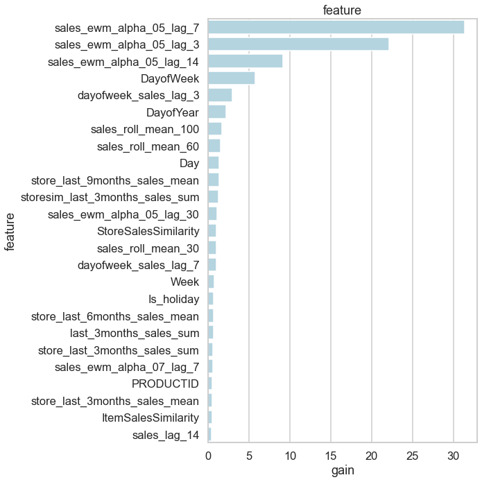
Feature Importance
def plot_lgb_importances(model, plot=False, num=10):
    from matplotlib import pyplot as plt
    import seaborn as sns


    # LGBM API
    #gain = model.feature_importance('gain')
    #feat_imp = pd.DataFrame({'feature': model.feature_name(),
    #                         'split': model.feature_importance('split'),
    #                         'gain': 100 * gain / gain.sum()}).sort_values('gain', ascending=False)

    # SKLEARN API
    gain = model.booster_.feature_importance(importance_type='gain')
    feat_imp = pd.DataFrame({'feature': model.feature_name_,
                             'split': model.booster_.feature_importance(importance_type='split'),
                             'gain': 100 * gain / gain.sum()}).sort_values('gain', ascending=False)
    if plot:
        plt.figure(figsize=(10, 10))
        sns.set_context("talk", font_scale=1)
        sns.set_style("whitegrid")
        sns.barplot(x="gain", y="feature", data=feat_imp[0:25], color = 'lightblue')
        plt.title('feature')
        plt.tight_layout()
        plt.show()
    else:
        print(feat_imp.head(num))
        return feat_imp

feature_imp_df = plot_lgb_importances(first_model, num=10)
                           feature  split       gain
141       sales_ewm_alpha_05_lag_7     78  31.387042
140       sales_ewm_alpha_05_lag_3    100  22.170319
142      sales_ewm_alpha_05_lag_14     51   9.177836
6                        DayofWeek    267   5.746324
114          dayofweek_sales_lag_3     76   2.918399
7                        DayofYear    190   2.184596
21             sales_roll_mean_100    204   1.659234
20              sales_roll_mean_60    173   1.539139
5                              Day    165   1.366325
43   store_last_9months_sales_mean      7   1.329502
feature_imp_df.shape, feature_imp_df[feature_imp_df.gain > 0].shape, feature_imp_df[feature_imp_df.gain > 0.57].shape
((151, 3), (133, 3), (21, 3))
plot_lgb_importances(first_model, plot=True)
Shap
SHAP (SHapley Additive exPlanations) is a game theoretic approach to explain the output of any machine learning model. It connects optimal credit allocation with local explanations using the classic Shapley values from game theory and their related extensions.
sns.set_context('talk', font_scale = 1.4)
explainer = shap.Explainer(first_model)
shap_values_train = explainer(X_train)
shap_values_valid = explainer(X_val)

len(shap_values_train), len(shap_values_valid)
(217822, 44368)
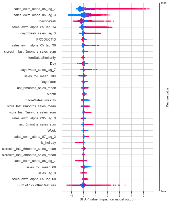
A beeswarm summary plot
The beeswarm plot is designed to display an information-dense summary of how the top features in a dataset impact the model’s output. Each instance the given explanation is represented by a single dot on each feature fow. The x position of the dot is determined by the SHAP value (shap_values.value[instance,feature]) of that feature, and dots “pile up” along each feature row to show density. Color is used to display the original value of a feature (shap_values.data[instance,feature]). In the plot below we can see that sales lag for 3 days is the most important feature on average for the training data. However, for the validation data sales lag for 7 days is the most important feature on average.
# summarize the effects of all the features
sns.set_context('talk', font_scale = 1.4)
shap.plots.beeswarm(shap_values_train, max_display=30)
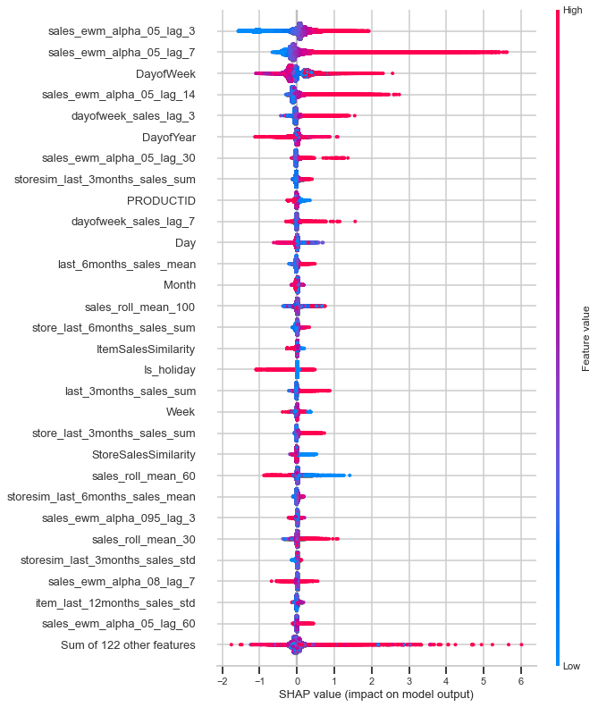
# summarize the effects of all the features
sns.set_context('talk', font_scale = 1.4)
shap.plots.beeswarm(shap_values_valid, max_display=30)
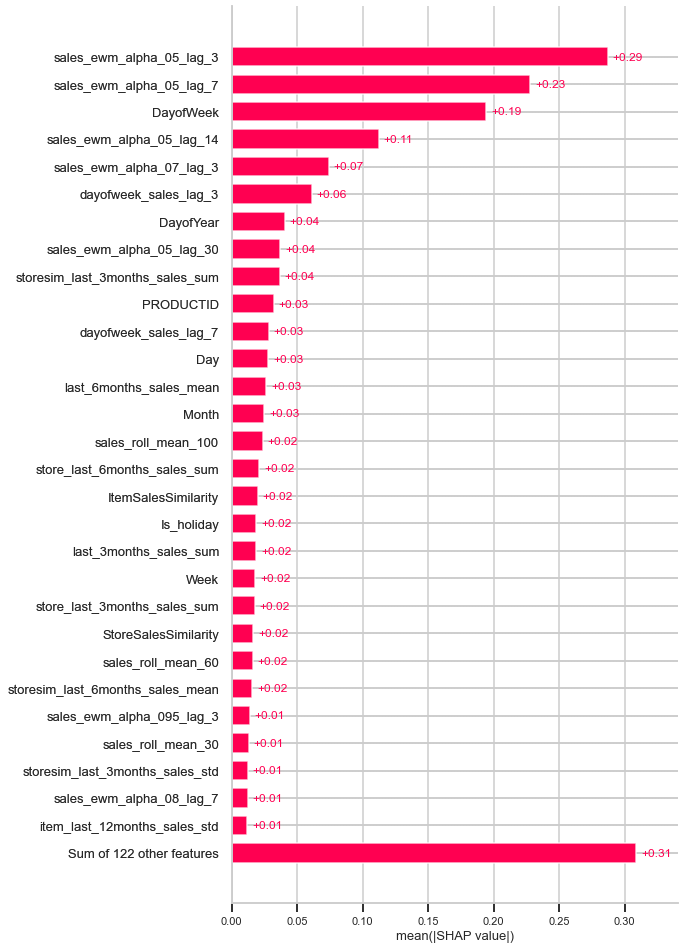
shap.plots.bar(shap_values_train, max_display=30)
Error Analysis
error = pd.DataFrame({
    "date":val.SALEDATE,
    "store":X_val.LOCATIONNO,
    "item":X_val.PRODUCTID,
    "actual":Y_val,
    "pred":first_model.predict(X_val)
}).reset_index(drop = True)

error["error"] = np.abs(error.actual-error.pred)

error.sort_values("error", ascending=False).head(20)
| date | store | item | actual | pred | error | |
|---|---|---|---|---|---|---|
| 38403 | 2021-02-21 | 30 | 41 | 85.0 | 11.357431 | 73.642569 |
| 38456 | 2021-02-21 | 30 | 37 | 57.0 | 9.129747 | 47.870253 |
| 38569 | 2021-02-21 | 30 | 3 | 59.0 | 13.590359 | 45.409641 |
| 38439 | 2021-02-21 | 4 | 41 | 36.0 | 5.282435 | 30.717565 |
| 18216 | 2021-01-25 | 30 | 42 | 43.0 | 13.941786 | 29.058214 |
| 39840 | 2021-02-22 | 30 | 42 | 38.0 | 9.921250 | 28.078750 |
| 43925 | 2021-02-28 | 30 | 41 | 44.0 | 16.407923 | 27.592077 |
| 14008 | 2021-01-19 | 30 | 42 | 32.0 | 8.389453 | 23.610547 |
| 38932 | 2021-02-21 | 4 | 37 | 31.0 | 7.826655 | 23.173345 |
| 38563 | 2021-02-21 | 30 | 43 | 31.0 | 8.182316 | 22.817684 |
| 39088 | 2021-02-21 | 36 | 3 | 29.0 | 7.635129 | 21.364871 |
| 41019 | 2021-02-24 | 30 | 3 | 26.0 | 4.827231 | 21.172769 |
| 29090 | 2021-02-08 | 30 | 41 | 32.0 | 11.175341 | 20.824659 |
| 22973 | 2021-01-31 | 12 | 42 | 30.0 | 9.534384 | 20.465616 |
| 40879 | 2021-02-24 | 30 | 27 | 25.0 | 4.890703 | 20.109297 |
| 8366 | 2021-01-12 | 30 | 27 | 29.0 | 9.047829 | 19.952171 |
| 23307 | 2021-01-31 | 30 | 41 | 35.0 | 15.066269 | 19.933731 |
| 28965 | 2021-02-08 | 4 | 37 | 26.0 | 6.205603 | 19.794397 |
| 27421 | 2021-02-06 | 30 | 27 | 27.0 | 7.547040 | 19.452960 |
| 35710 | 2021-02-17 | 32 | 41 | 25.0 | 5.810368 | 19.189632 |
error[["actual", "pred", "error"]].describe([0.7, 0.8, 0.9, 0.95, 0.99]).T
| count | mean | std | min | 50% | 70% | 80% | 90% | 95% | 99% | max | |
|---|---|---|---|---|---|---|---|---|---|---|---|
| actual | 44368.0 | 2.584691 | 3.101834 | 0.000000 | 2.000000 | 3.000000 | 4.000000 | 6.000000 | 8.000000 | 14.000000 | 85.000000 |
| pred | 44368.0 | 2.350267 | 1.485043 | 0.101703 | 2.007167 | 2.537990 | 2.980707 | 3.834862 | 4.929053 | 8.650099 | 18.277589 |
| error | 44368.0 | 1.864230 | 1.917119 | 0.000021 | 1.405939 | 2.089352 | 2.657121 | 3.826397 | 5.232841 | 9.339638 | 73.642569 |
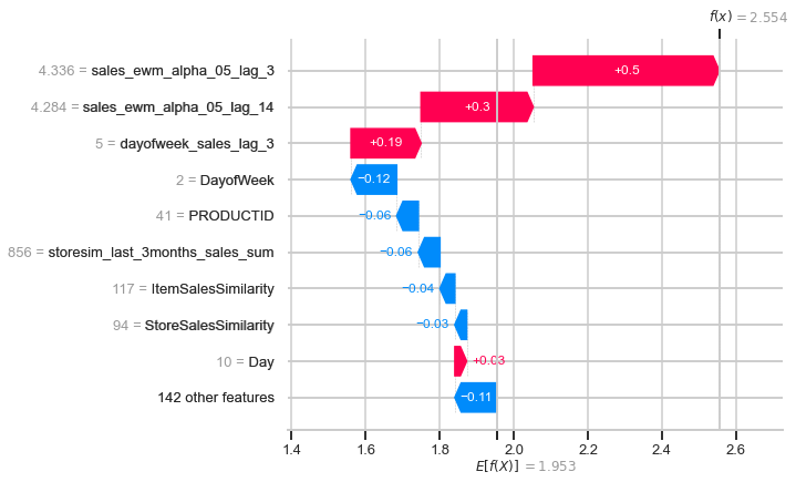
Waterfall plots are designed to display explanations for individual predictions, so they expect a single row of an Explanation object as input. The bottom of a waterfall plot starts as the expected value of the model output, and then each row shows how the positive (red) or negative (blue) contribution of each feature moves the value from the expected model output over the background dataset to the model output for this prediction.
sns.set_context('talk', font_scale = 1.4)
shap.plots.waterfall(shap_values_valid[30125])
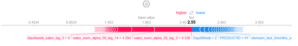
Force plot is used to show how much a given feature contributes to our prediction (compared to if we made that prediction at some baseline value of that feature). The force plots are interactive, as github had difficulty rendering it; I have uploaded the pictures of the plots.
# visualize the first prediction's explanation with a force plot
shap.initjs()
shap.plots.force(shap_values_valid[30125])
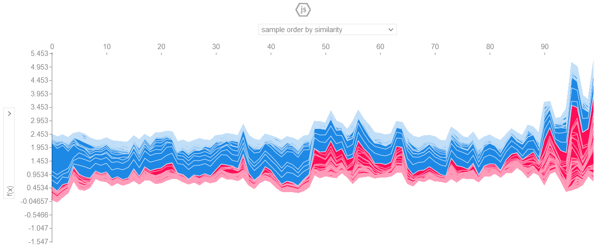
# visualize the explanation for the all the prediction with a force plot. So as to not overwhelm the browser
# first 100 values are passed
valid_shap = explainer.shap_values(X_val)
shap.initjs()
shap.plots.force(explainer.expected_value, valid_shap[:100, :], X_val.iloc[:100, :])
# Mean Absolute Error
error.groupby(["store", "item"]).error.mean().sort_values(ascending = False)
store item
30 41 8.796683
3 7.730369
27 7.417767
42 7.331254
37 6.566694
1 6.551101
38 6.450013
8 5.688377
34 5.215296
11 4.847538
43 4.786728
12 42 4.604071
3 4.430166
30 13 4.366960
40 4.349082
0 34 4.321580
42 4.259871
30 39 4.251495
4 37 4.141325
8 4.049376
33 3 3.985145
4 42 3.982138
12 8 3.964201
27 3.933068
0 11 3.931204
3 3.796247
1 3.767996
12 34 3.690778
0 27 3.663062
30 44 3.632818
12 41 3.628897
4 3 3.591541
0 8 3.581333
4 41 3.575084
24 1 3.554002
0 41 3.517047
1 3 3.429900
4 38 3.424165
1 3.372646
27 3.366829
36 3 3.359900
33 8 3.340034
1 3.331595
30 45 3.328554
14 41 3.318947
27 3 3.310898
39 42 3.283005
33 38 3.237391
39 1 3.190325
17 27 3.186373
32 41 3.174905
33 27 3.141269
4 13 3.132354
12 38 3.108171
11 3.100573
19 3 3.097261
39 27 3.074528
24 42 3.071504
12 13 3.059989
0 44 2.998813
33 11 2.953767
42 1 2.942637
12 1 2.926406
14 38 2.910530
0 43 2.908644
2 13 2.896304
33 34 2.895418
42 13 2.895023
4 39 2.891847
33 41 2.886471
39 3 2.878725
0 37 2.872639
12 44 2.863298
15 41 2.859410
27 43 2.835657
14 34 2.831470
12 43 2.803658
2 42 2.795462
19 38 2.767300
17 8 2.758636
12 40 2.756067
14 42 2.754917
17 1 2.754808
34 2.743868
33 44 2.742895
24 43 2.742398
8 41 2.708218
18 1 2.701318
17 38 2.678119
1 27 2.665648
14 37 2.664356
3 41 2.661593
42 3 2.646940
19 27 2.634222
27 42 2.632597
27 2.621078
2 8 2.599549
16 1 2.599387
14 8 2.591194
32 11 2.586096
0 38 2.585180
32 37 2.580516
15 37 2.577988
19 41 2.577918
24 38 2.572516
2 27 2.558549
0 13 2.553786
24 13 2.549550
32 8 2.541285
7 38 2.538866
39 37 2.534707
41 2.533105
36 41 2.526091
42 2.524357
4 43 2.523554
24 27 2.517807
12 39 2.514400
37 2.510257
32 3 2.495721
7 3 2.472591
32 27 2.472559
42 37 2.471904
27 1 2.468068
33 39 2.466154
16 41 2.456669
27 41 2.455888
13 2.454431
17 44 2.451902
42 41 2.436222
24 41 2.427852
26 3 2.425128
15 42 2.423113
33 37 2.413726
2 1 2.412799
17 3 2.410413
0 45 2.398012
24 3 2.396723
32 42 2.390878
1 1 2.364970
7 41 2.363477
24 8 2.363074
2 3 2.360506
19 42 2.349965
24 37 2.349415
19 37 2.346062
18 11 2.344202
32 38 2.340597
7 37 2.332521
4 34 2.330637
33 42 2.328101
32 34 2.319122
14 27 2.315701
16 3 2.286446
15 27 2.285725
42 27 2.272444
1 8 2.258241
36 39 2.254372
21 42 2.237494
27 38 2.237187
16 27 2.231148
18 3 2.228452
42 11 2.226240
19 1 2.223807
36 37 2.216599
39 11 2.212751
3 3 2.209608
44 3 2.205291
19 8 2.202903
26 8 2.193774
1 44 2.187075
17 13 2.183657
25 1 2.183614
1 37 2.175282
21 38 2.171630
39 43 2.163067
3 37 2.157286
19 34 2.152494
1 11 2.149056
15 3 2.147725
17 43 2.134811
27 11 2.134671
1 38 2.134429
15 38 2.134370
8 42 2.130037
19 11 2.126680
36 27 2.125526
42 42 2.116560
7 1 2.115409
32 13 2.114694
1 42 2.113248
2 43 2.112902
42 38 2.108225
18 41 2.104434
16 42 2.101756
20 8 2.094922
23 3 2.089880
38 1 2.088971
18 42 2.083530
27 8 2.076874
44 43 2.066242
45 37 2.066145
15 1 2.066116
21 13 2.064104
39 8 2.063827
28 41 2.062566
0 40 2.060275
4 11 2.059599
17 42 2.058140
3 42 2.057786
38 3 2.054505
8 37 2.051368
43 42 2.041615
40 37 2.038056
33 13 2.035505
14 3 2.033955
8 3 2.033846
22 42 2.033555
36 13 2.029968
24 34 2.029384
16 38 2.027139
1 43 2.024892
26 41 2.024144
16 8 2.022475
11 41 2.012826
26 37 2.008662
13 2.003392
44 1 1.999507
5 42 1.997661
1 13 1.996955
44 44 1.996313
10 41 1.989540
40 3 1.987509
25 42 1.984760
26 1 1.984527
1 41 1.978309
33 43 1.973729
17 41 1.973248
26 34 1.973114
41 27 1.970733
21 37 1.962348
3 1 1.960896
23 8 1.960636
44 42 1.957164
3 38 1.956553
42 43 1.949328
18 37 1.949230
39 13 1.948035
44 41 1.945350
20 41 1.945303
18 34 1.940320
44 8 1.940279
17 37 1.935355
33 40 1.933901
3 43 1.933638
25 3 1.932040
24 40 1.927933
6 42 1.927292
22 8 1.926427
39 44 1.917073
4 45 1.915448
26 27 1.915327
42 40 1.912418
27 34 1.912250
42 8 1.911520
3 8 1.909868
19 43 1.909620
39 38 1.908371
2 37 1.907649
18 27 1.902842
6 41 1.901781
3 11 1.896718
36 1 1.889901
44 27 1.886836
1 39 1.881931
36 8 1.873640
14 43 1.872762
26 38 1.871297
45 44 1.865992
39 39 1.865921
44 13 1.864748
27 45 1.863641
42 44 1.862351
21 1 1.859969
41 1 1.858548
15 34 1.858174
25 8 1.857868
2 34 1.857595
0 39 1.856275
20 34 1.851778
32 40 1.848275
24 44 1.845841
43 3 1.843875
31 41 1.843710
19 13 1.842873
17 11 1.842854
3 34 1.839337
21 43 1.838972
8 38 1.835077
43 13 1.824492
18 38 1.820752
25 41 1.820603
2 41 1.814130
14 39 1.813962
3 13 1.813783
20 13 1.813201
35 34 1.811165
20 27 1.810796
10 27 1.803908
14 44 1.801503
2 38 1.798955
6 34 1.798940
42 39 1.798875
45 27 1.796934
21 11 1.796591
36 11 1.793527
35 38 1.790625
8 34 1.790520
5 38 1.790312
21 39 1.787890
31 38 1.787751
7 8 1.783308
14 1 1.783071
24 39 1.781381
15 8 1.776310
9 41 1.768692
25 13 1.761052
10 3 1.760061
16 11 1.753975
28 37 1.752716
36 38 1.751559
6 1 1.748578
7 34 1.744266
38 37 1.743989
39 40 1.741437
18 13 1.737523
42 34 1.736864
2 40 1.735879
10 34 1.732812
32 1 1.730147
8 1 1.729259
3 27 1.728229
32 39 1.727863
16 44 1.726095
20 1 1.725890
40 42 1.724510
1 34 1.721047
25 34 1.710974
19 44 1.710354
26 44 1.707571
44 37 1.707304
32 44 1.705164
21 8 1.697304
38 27 1.693728
22 43 1.692139
45 38 1.691840
28 8 1.691809
20 42 1.690213
41 41 1.690204
45 11 1.688956
21 41 1.687332
15 43 1.683894
10 8 1.681712
46 27 1.678961
33 45 1.677837
22 13 1.669968
21 27 1.669549
37 3 1.667952
29 1 1.664966
39 34 1.664316
19 39 1.662362
36 43 1.660920
35 41 1.658878
38 11 1.658647
20 44 1.655116
7 42 1.653392
4 44 1.650880
35 42 1.649943
41 37 1.643977
22 27 1.642987
41 42 1.641927
14 13 1.639081
35 3 1.637331
28 42 1.635993
26 42 1.635693
36 34 1.633226
21 3 1.631875
23 27 1.629565
13 42 1.629360
41 3 1.629063
6 38 1.628237
2 11 1.625523
46 42 1.625001
39 45 1.624650
31 34 1.624203
43 8 1.622206
45 3 1.617795
2 44 1.616223
5 1 1.615027
3 1.611376
17 45 1.609809
6 3 1.608170
16 13 1.605829
17 39 1.605315
10 42 1.605111
44 34 1.604073
26 40 1.602739
8 8 1.601100
20 3 1.600886
37 42 1.599365
46 1 1.599363
7 11 1.595823
19 40 1.595275
25 37 1.594842
3 39 1.594068
27 44 1.592834
28 38 1.591825
4 40 1.591698
15 40 1.589640
40 11 1.589380
43 1 1.588752
8 13 1.588291
27 1.587870
20 37 1.586954
40 27 1.585805
1 1.582457
35 43 1.580955
44 39 1.580266
6 37 1.580047
10 40 1.571123
23 1 1.570028
38 43 1.569349
8 43 1.566729
27 37 1.566515
45 41 1.563603
21 44 1.563534
27 39 1.558764
29 42 1.557502
45 42 1.557341
18 39 1.555327
17 40 1.553271
18 44 1.553210
26 11 1.552130
36 45 1.551781
31 37 1.548940
10 38 1.542138
25 38 1.536770
3 45 1.533392
14 11 1.533245
11 42 1.533169
41 13 1.531229
22 41 1.531058
6 27 1.530885
31 27 1.529504
22 3 1.528377
25 44 1.526525
44 38 1.522776
15 13 1.522659
23 42 1.522417
18 40 1.516749
35 27 1.516605
26 39 1.516518
9 37 1.515547
27 40 1.514145
18 43 1.506296
26 43 1.501951
22 34 1.501277
9 8 1.501055
31 8 1.497446
36 44 1.494615
46 8 1.488384
37 27 1.485193
20 39 1.482098
13 38 1.480978
45 40 1.477098
31 3 1.476729
5 37 1.476702
15 39 1.473841
20 43 1.472823
25 40 1.472325
43 41 1.471055
25 43 1.470083
11 1.469726
29 38 1.467283
35 44 1.465114
19 45 1.461398
29 13 1.459881
38 42 1.459658
45 1 1.456833
43 43 1.455565
6 8 1.454127
13 41 1.453342
20 11 1.453098
41 8 1.452080
13 8 1.441653
11 3 1.439156
25 27 1.435201
24 11 1.434468
18 8 1.434382
9 38 1.433600
28 3 1.433528
31 13 1.425882
16 43 1.425030
5 34 1.419403
24 45 1.417889
32 45 1.413463
14 45 1.413133
28 1 1.409939
32 43 1.409382
36 40 1.408973
40 38 1.408733
41 1.406929
38 8 1.406324
35 1 1.404390
8 40 1.403327
46 39 1.397547
13 1 1.396676
35 8 1.393965
15 44 1.392225
46 41 1.390153
38 38 1.386612
46 43 1.384864
9 34 1.383108
34 27 1.383070
11 38 1.382509
6 44 1.381311
21 34 1.381135
11 1 1.380937
6 45 1.380672
41 44 1.379753
7 27 1.377542
10 44 1.376408
45 34 1.372226
22 37 1.371057
11 27 1.370857
34 1.364955
42 45 1.364858
23 37 1.364523
37 38 1.364031
44 11 1.362768
28 27 1.356454
16 34 1.355161
23 38 1.351869
43 11 1.350829
3 44 1.349670
10 11 1.347824
7 13 1.346960
10 13 1.346377
5 41 1.346221
13 27 1.344241
3 1.343940
43 27 1.343367
44 40 1.341989
46 3 1.337838
13 34 1.335442
38 40 1.331371
20 38 1.331275
1 40 1.325123
46 37 1.319289
29 41 1.318189
26 45 1.317941
35 37 1.316348
15 11 1.310689
28 43 1.307173
23 13 1.303640
15 45 1.303377
12 45 1.301729
35 13 1.300401
21 45 1.300292
14 40 1.298674
41 43 1.297476
10 1 1.297088
20 40 1.290303
40 39 1.288799
46 13 1.288330
10 39 1.286495
9 27 1.286425
8 44 1.285620
44 45 1.285025
22 40 1.280695
5 13 1.279332
29 37 1.278220
13 13 1.277620
31 44 1.277343
5 40 1.275691
2 39 1.275454
8 11 1.273474
23 41 1.272285
1 45 1.271653
16 37 1.271520
41 11 1.267283
31 42 1.265529
23 34 1.265441
46 11 1.263586
10 37 1.263164
22 44 1.262131
41 38 1.261945
40 43 1.261918
37 43 1.261241
40 13 1.260632
37 41 1.258518
11 11 1.254279
13 45 1.251213
8 39 1.244513
43 37 1.241200
38 39 1.240999
2 45 1.240259
22 1 1.235999
45 43 1.235887
13 44 1.229849
41 39 1.229810
37 11 1.228697
40 8 1.223290
23 11 1.220861
41 40 1.220079
22 38 1.217430
40 44 1.215226
5 11 1.211048
11 13 1.209994
35 39 1.209714
40 34 1.207613
23 39 1.205320
7 44 1.203008
6 40 1.199670
43 1.199251
34 38 1.190904
6 11 1.190330
29 39 1.189879
22 45 1.186641
34 1 1.186173
25 45 1.180808
11 40 1.180772
28 34 1.179983
38 44 1.179506
11 44 1.176823
43 44 1.175224
31 11 1.169490
28 11 1.168184
38 13 1.167285
35 40 1.161437
29 43 1.159207
8 45 1.157875
29 40 1.156590
9 1 1.153502
16 39 1.149489
46 44 1.148087
21 40 1.146468
18 45 1.146364
6 13 1.144507
10 43 1.138214
28 40 1.135324
23 43 1.129761
41 34 1.121338
38 41 1.121165
7 40 1.120401
16 40 1.118409
23 40 1.115234
38 45 1.114810
5 8 1.113851
20 45 1.111943
5 27 1.102829
13 37 1.101488
40 1.100397
43 34 1.100327
37 13 1.100285
34 42 1.098209
28 44 1.095334
11 37 1.094298
45 13 1.093022
28 39 1.092296
38 34 1.092063
31 1 1.087255
28 13 1.086889
3 40 1.083108
37 1 1.082157
9 3 1.081618
29 11 1.078017
5 44 1.074451
45 45 1.072343
39 1.069386
34 11 1.066682
46 38 1.065999
29 27 1.065617
34 34 1.065393
43 38 1.062559
37 37 1.059753
7 45 1.059462
6 39 1.058750
7 43 1.058048
29 8 1.055055
25 39 1.053514
13 11 1.052914
29 34 1.050733
10 45 1.049201
31 39 1.048510
16 45 1.046897
37 44 1.038964
29 3 1.038124
46 34 1.037908
29 45 1.037392
22 11 1.034675
7 39 1.032651
23 44 1.025163
45 8 1.020356
35 45 1.011467
46 40 1.010654
37 34 1.009384
34 13 1.004393
46 45 1.003513
29 44 0.995035
37 8 0.993700
31 40 0.987735
34 8 0.982164
40 40 0.980587
41 45 0.980504
31 45 0.970299
37 40 0.967668
9 13 0.953869
34 37 0.950879
13 39 0.948704
28 45 0.946098
13 43 0.936056
31 43 0.929694
37 39 0.929275
23 45 0.928652
34 41 0.927818
40 45 0.917975
35 11 0.905323
37 45 0.903277
9 42 0.902879
34 44 0.901609
43 0.897353
22 39 0.888240
11 8 0.887651
5 43 0.865483
39 0.857759
34 45 0.853622
40 0.847206
9 39 0.844469
11 0.843750
5 45 0.842548
43 45 0.832047
9 44 0.808320
43 40 0.807350
34 3 0.802921
43 39 0.792631
34 39 0.789006
11 39 0.730254
9 43 0.719432
11 45 0.704662
9 40 0.702955
11 43 0.697794
9 45 0.670643
Name: error, dtype: float64
# Mean Absolute Error
error.groupby(["item"]).error.mean().sort_values(ascending = False)
item
3     2.300384
41    2.237997
42    2.224660
27    2.125854
1     2.119102
8     1.999352
38    1.992689
37    1.982540
34    1.842083
13    1.798909
11    1.722505
43    1.682012
44    1.597961
39    1.484561
40    1.441437
45    1.275640
Name: error, dtype: float64
# Store 1 Actual - Pred
sns.set_context("talk", font_scale=1.4)
# fig, axes = plt.subplots(8, 6, figsize=(20, 35))
sub = error[error.store == 1].set_index("date")
fig, axes = plt.subplots(8, 6, figsize=(30, 40))
for i in range(0,46):
    if i < 6:
        sub[sub.item == i].actual.plot(ax=axes[0, i], legend=True, label = "Item "+str(i)+" Sales")
        sub[sub.item == i].pred.plot(ax=axes[0, i], legend=True, label="Item " + str(i) + " Pred", linestyle = "dashed")
    elif i > 5 and i < 12:
        sub[sub.item == i].actual.plot(ax=axes[1, i - 6], legend=True, label = "Item "+str(i)+" Sales")
        sub[sub.item == i].pred.plot(ax=axes[1, i - 6], legend=True, label="Item " + str(i) + " Pred",  linestyle="dashed")
    elif i > 11 and i< 18:
        sub[sub.item == i].actual.plot(ax=axes[2, i - 12], legend=True, label = "Item "+str(i)+" Sales")
        sub[sub.item == i].pred.plot(ax=axes[2, i - 12], legend=True, label="Item " + str(i) + " Pred", linestyle="dashed")
    elif i > 17 and i< 24:
        sub[sub.item == i].actual.plot(ax=axes[3, i - 18], legend=True, label = "Item "+str(i)+" Sales")
        sub[sub.item == i].pred.plot(ax=axes[3, i - 18], legend=True, label="Item " + str(i) + " Pred", linestyle="dashed")
    elif i > 23 and i< 30:
        sub[sub.item == i].actual.plot(ax=axes[4, i - 24], legend=True, label = "Item "+str(i)+" Sales")
        sub[sub.item == i].pred.plot(ax=axes[4, i - 24], legend=True, label="Item " + str(i) + " Pred", linestyle="dashed")
    elif i > 29 and i< 36:
        sub[sub.item == i].actual.plot(ax=axes[5, i - 30], legend=True, label = "Item "+str(i)+" Sales")
        sub[sub.item == i].pred.plot(ax=axes[5, i - 30], legend=True, label="Item " + str(i) + " Pred", linestyle="dashed")
    elif i > 35 and i < 42:
        sub[sub.item == i].actual.plot(ax=axes[6, i - 36], legend=True, label = "Item "+str(i)+" Sales")
        sub[sub.item == i].pred.plot(ax=axes[6, i - 36], legend=True, label="Item " + str(i) + " Pred", linestyle="dashed")
    else:
        sub[sub.item == i].actual.plot(ax=axes[7, i - 42], legend=True, label = "Item "+str(i)+" Sales")
        sub[sub.item == i].pred.plot(ax=axes[7, i - 42], legend=True, label="Item " + str(i) + " Pred", linestyle="dashed")

plt.tight_layout(pad=3)
plt.suptitle("Store 1 Items");
plt.show()
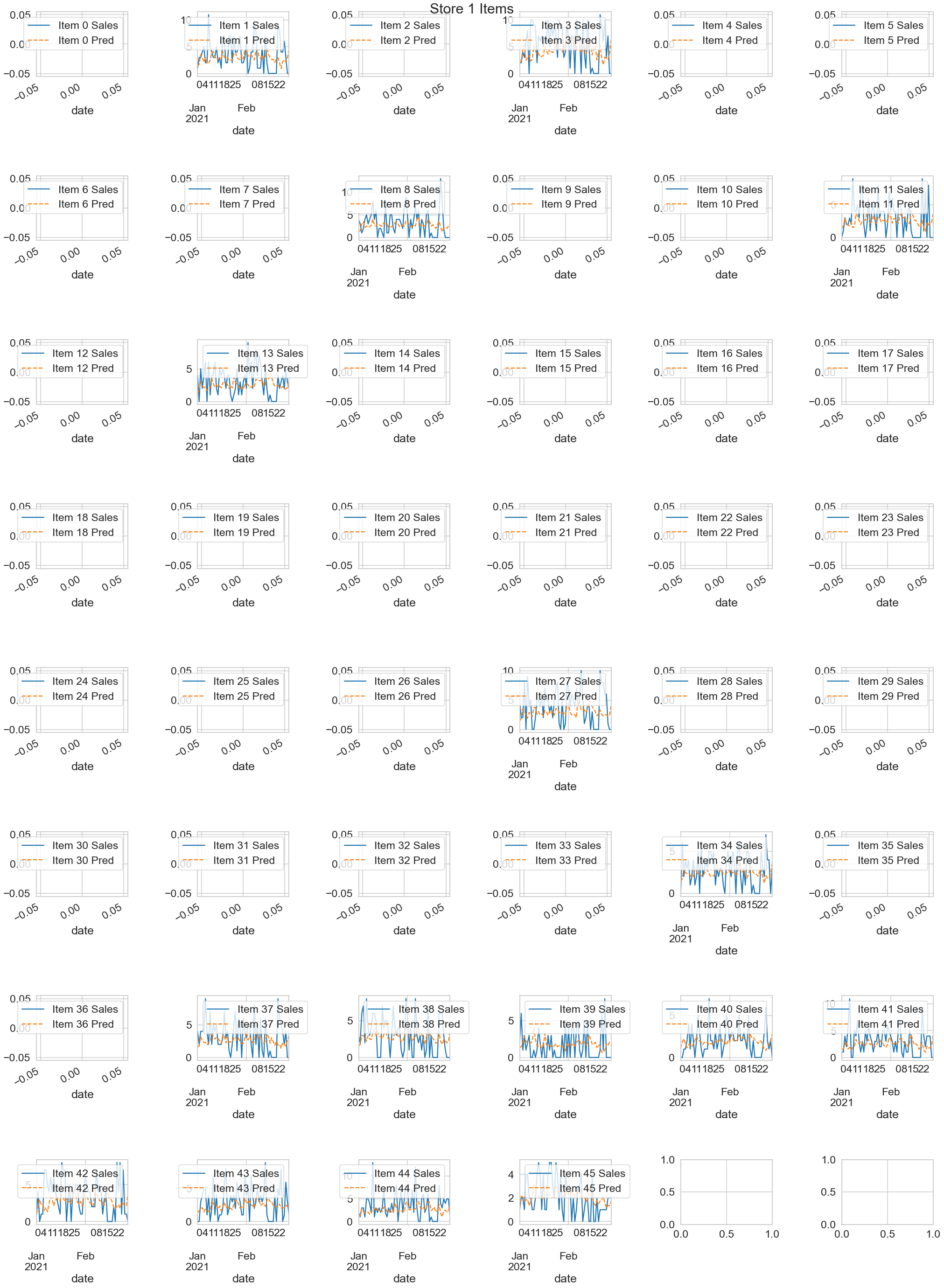
sns.set_context('talk', font_scale = 1.4)
fig, axes = plt.subplots(4, 2, figsize = (20,20))
for axi in axes.flat:
    axi.ticklabel_format(style="sci", axis="y", scilimits=(0,10))
    axi.ticklabel_format(style="sci", axis="x", scilimits=(0,10))
    axi.get_yaxis().set_major_formatter(plt.FuncFormatter(lambda x, loc: "{:,}".format(int(x))))
    axi.get_xaxis().set_major_formatter(plt.FuncFormatter(lambda x, loc: "{:,}".format(int(x))))

(error.actual-error.pred).hist(ax = axes[0, 0], color = "steelblue", bins = 20)
error.error.hist(ax = axes[0,1], color = "steelblue", bins = 20)
sr = error.copy()
sr["StandardizedR"] = (sr.error / (sr.actual-sr.pred).std())
sr["StandardizedR2"] = ((sr.error / (sr.actual-sr.pred).std())**2)
sr.plot.scatter(x = "pred",y = "StandardizedR", color = "red", ax = axes[1,0])
sr.plot.scatter(x = "pred",y = "StandardizedR2", color = "red", ax = axes[1,1])
error.actual.hist(ax = axes[2, 0], color = "purple", bins = 20)
error.pred.hist(ax = axes[2, 1], color = "purple", bins = 20)
error.plot.scatter(x = "actual",y = "pred", color = "seagreen", ax = axes[3,0]);

# QQ Plot
import statsmodels.api as sm
import pylab
sm.qqplot(sr.pred, ax = axes[3,1], c = "seagreen")
plt.suptitle("ERROR ANALYSIS", fontsize = 20)
axes[0,0].set_title("Error Histogram", fontsize = 15)
axes[0,1].set_title("Absolute Error Histogram", fontsize = 15)
axes[1,0].set_title("Standardized Residuals & Fitted Values", fontsize = 15)
axes[1,1].set_title("Standardized Residuals^2 & Fitted Values", fontsize = 15)
axes[2,0].set_title("Actual Histogram", fontsize = 15)
axes[2,1].set_title("Pred Histogram", fontsize = 15);
axes[3,0].set_title("Actual Pred Relationship", fontsize = 15);
axes[3,1].set_title("QQ Plot", fontsize = 15);
axes[1,0].set_xlabel("Fitted Values (Pred)", fontsize = 12)
axes[1,1].set_xlabel("Fitted Values (Pred)", fontsize = 12)
axes[3,0].set_xlabel("Actual", fontsize = 12)
axes[1,0].set_ylabel("Standardized Residuals", fontsize = 12)
axes[1,1].set_ylabel("Standardized Residuals^2", fontsize = 12)
axes[3,0].set_ylabel("Pred", fontsize = 12)
fig.tight_layout(pad=3.0)
plt.savefig("errors.png")
plt.show()
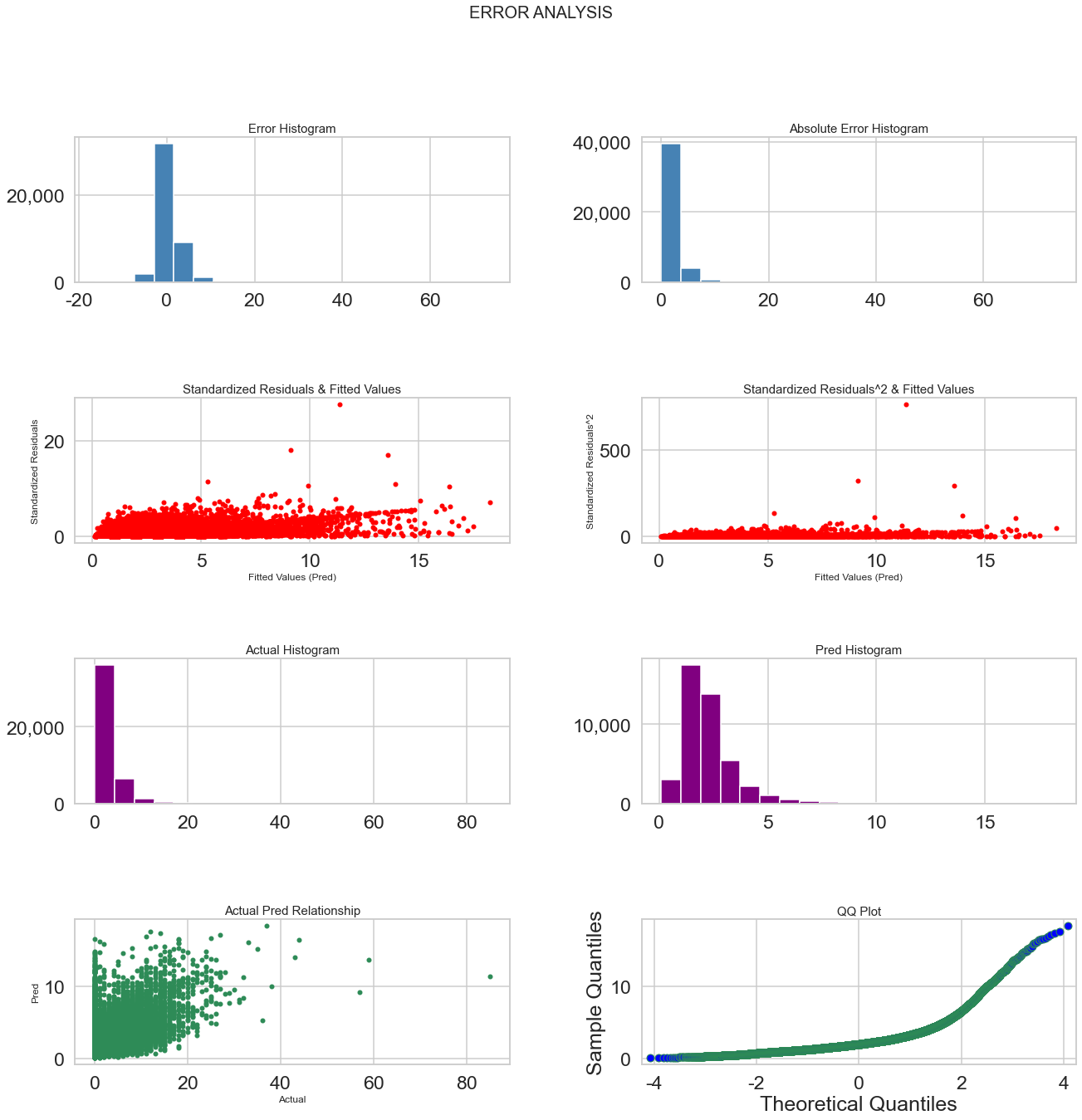
Next Model
Default Parameters & Feature Selection with LGBM Feature Importance
# First model feature importance
cols = feature_imp_df[feature_imp_df.gain > 0.015].feature.tolist()
print("Independent Variables:", len(cols))

second_model = lgb.LGBMRegressor(random_state=384).fit(
    X_train[cols], Y_train,
    eval_metric = lambda y_true, y_pred: [lgbm_smape(y_true, y_pred)])

print("TRAIN SMAPE:", smape(Y_train, second_model.predict(X_train[cols])))
print("VALID SMAPE:", smape(Y_val, second_model.predict(X_val[cols])))
Independent Variables: 117
TRAIN SMAPE: 69.48193950896932
VALID SMAPE: 95.93174397344767
lgbm_params = {

"num_leaves":[20,31], # Default 31
"max_depth":[-1, 20, 30], # Default -1
"learning_rate":[0.1, 0.05], # Default 0.1
"n_estimators":[10000,15000], # Default 100
"min_split_gain":[0.0, 2,5], # Default 0
"min_child_samples":[10, 20, 30], # Default 20
"colsample_bytree":[0.5, 0.8, 1.0], # Default 1
"reg_alpha":[0.0, 0.5, 1], # Default 0
"reg_lambda":[0.0, 0.5, 1] # Default 0

}

model = lgb.LGBMRegressor(random_state=384)

tscv = TimeSeriesSplit(n_splits=3)
rsearch = RandomizedSearchCV(model, lgbm_params, random_state=384, cv=tscv, scoring=make_scorer(smape), verbose = True, n_jobs = -1).fit( X_train[cols], Y_train )

print(rsearch.best_params_)
Fitting 3 folds for each of 10 candidates, totalling 30 fits


[Parallel(n_jobs=-1)]: Using backend LokyBackend with 8 concurrent workers.
[Parallel(n_jobs=-1)]: Done  30 out of  30 | elapsed: 142.9min finished


{'reg_lambda': 0.0, 'reg_alpha': 1, 'num_leaves': 20, 'n_estimators': 10000, 'min_split_gain': 0.0, 'min_child_samples': 20, 'max_depth': 20, 'learning_rate': 0.1, 'colsample_bytree': 1.0}
model_tuned = lgb.LGBMRegressor(**rsearch.best_params_, random_state=384).fit(X_train[cols], Y_train)

print("TRAIN SMAPE:", smape(Y_train, model_tuned.predict(X_train[cols])))
print("VALID SMAPE:", smape(Y_val, model_tuned.predict(X_val[cols])))
TRAIN SMAPE: 48.433166801003026
VALID SMAPE: 97.24837091281393
model_tuned2 = lgb.LGBMRegressor(num_leaves=31, n_estimators=15000, max_depth=20, random_state=384, metric = "custom")
model_tuned2.fit(
    X_train[cols], Y_train,
    eval_metric= lambda y_true, y_pred: [lgbm_smape(y_true, y_pred)],
    eval_set = [(X_train[cols], Y_train), (X_val[cols], Y_val)],
    eval_names = ["Train", "Valid"],
    early_stopping_rounds= 1000, verbose = 500
)
print("Best Iteration:", model_tuned2.booster_.best_iteration)
Training until validation scores don't improve for 1000 rounds
[500]   Train's SMAPE: 66.2324  Valid's SMAPE: 95.4403
[1000]  Train's SMAPE: 63.2125  Valid's SMAPE: 95.5624
[1500]  Train's SMAPE: 60.7468  Valid's SMAPE: 95.4656
Early stopping, best iteration is:
[696]   Train's SMAPE: 64.8907  Valid's SMAPE: 95.3564
Best Iteration: 696
df.sort_values(["LOCATIONNO", "PRODUCTID", "SALEDATE"], inplace = True)

train_final = df.loc[(df["SALEDATE"] < "2021-03-01"), :]
test_final = df.loc[(df["SALEDATE"] >= "2021-03-01"), :]

X_train_final = train_final[cols]
Y_train_final = train_final.UNIT_GROSS_SALES
X_test_final = test_final[cols]


final_model = lgb.LGBMRegressor(num_leaves=31, n_estimators=15000, max_depth=20, random_state=384, metric = "custom")
final_model.set_params(n_estimators=model_tuned2.booster_.best_iteration) # Best Iteration: 983
final_model.fit(X_train_final[cols], Y_train_final,
                eval_metric= lambda y_true, y_pred: [lgbm_smape(y_true, y_pred)])
LGBMRegressor(max_depth=20, metric='custom', n_estimators=696, random_state=384)
final_model.predict(X_test_final)
array([6.82137589, 5.82712452, 3.76803532, ..., 2.00950222, 1.83432827,
       1.17740984])
sales_test = test_final[['LOCATIONNO', 'SALEDATE', 'PRODUCTID', 'UNIT_GROSS_SALES']]
sales_test['Predictions'] = np.round(final_model.predict(X_test_final))
sales_test['error'] = sales_test['UNIT_GROSS_SALES'] - sales_test['Predictions']
sales_test.head()
| LOCATIONNO | SALEDATE | PRODUCTID | UNIT_GROSS_SALES | Predictions | error | |
|---|---|---|---|---|---|---|
| 262726 | 0 | 2021-03-01 | 1 | 6.0 | 7.0 | -1.0 |
| 263527 | 0 | 2021-03-02 | 1 | 12.0 | 6.0 | 6.0 |
| 264122 | 0 | 2021-03-03 | 1 | 1.0 | 4.0 | -3.0 |
| 264932 | 0 | 2021-03-04 | 1 | 4.0 | 4.0 | 0.0 |
| 265271 | 0 | 2021-03-05 | 1 | 6.0 | 3.0 | 3.0 |
item1 = sales_test[(sales_test['LOCATIONNO'] == 1) & (sales_test['PRODUCTID'] == 34)][['UNIT_GROSS_SALES', 'Predictions', 'error']]
sns.lineplot(data=item1, palette="tab10", linewidth=2.5)

plt.legend(bbox_to_anchor=(1.05, 1), loc='upper left')
<matplotlib.legend.Legend at 0x2ac01a5f8b0>

Future Work
The next step in the process is to utilize the news vendor model to estimate demand in each store for each item. A simulation can then be run to identify how many deliveries should be schedled throughout the week to minimize waste.