This project is focused on fitting an extended SIR model with time-dependent $R_0$-values and resource-dependent death rates to real Coronavirus data, in order to come as close as possible to the real numbers and make informed predictions about possible future developments. But before we jump right into fitting the data to our model, let’s do something that is often overlooked — let’s have a short look at what our model cannot do.
Caveats, Pitfalls, Limitations
Models are always simplifications of the real world. Still — that does not mean that they cannot be interesting and generate insights. It’s just important to keep the following things in mind:
The System of Differential Equations is extremely sensitive to initial parameters; Slight changes can lead to completely different outcomes.
We are extrapolating from incomplete, preliminary data. Some countries might only count deaths directly resulting from Coronavirus, others might count all deaths where the individual was infected. Some might (purposely or not) report inaccurate or unreliable data, etc.
We assume homogeneity among the whole population, that is, we do not account for some places being initial hot spots and others implementing restrictions earlier and more strenuously (we’d need much more effort (computationally and mathematically) to take these things into account).
Additionally, specific to our model, we make the following assumptions
Deaths do not change the population structure to a meaningful extent (we calculate fatality rates a priori (using the population structure from before the outbreak) and assume that deaths are not so high as to significantly change the population structure (I believe that this is a rather weak, reasonable assumption)).
Only critical cases fill up the hospitals and can lead to a higher fatality rate due to shortage of available care.
All critical patients that do not get treatment die.
Individuals are immune after recovering (This seems likely at the moment, at least for the vast majority of patients).
$R_0$ only decreases or stays constant. It does not increase. (Thus, this model does not allow us to model measures being loosened again; we’d need a different function for $R_0$ for that)
We will add jus one new compartment: Critical, for individuals that need intensive care. This will allow us to model overflowing hospitals. Of course, only infected individuals can enter the critical state. From the critical state, they can either die or recover.
We arrive at these transitions:

We need the probability that an infected individual becomes critically ill. We’ll just call it p(I→C). Logically, the probability of going from infected to recovered is thus 1-p(I→C). We need another probability, the probability of dying while critical: p(C→D). Analogously, the probability of going from infected to recovered is 1-p(C→D).
Now we’re only missing the rate of becoming critically ill after being infected, the rate of dying while being critically ill, and the rate of recovery while being critically ill. Reading through current estimates, we get the following numbers (These estimtes were aggregated from multiple sources, feel free to use different numbers; there should be more accurate numbers over time):
- Number of days from infected to critical: 12 (→rate: 1⁄12)
- Number of days from critical to dead: 7.5 (→rate: 1⁄7.5)
- Number of days from critical to recovered: 6.5 (→rate: 1⁄6.5)
Filling all this in:

Triage and Limited Resources
There has been lots of coverage on triage taking place in Italy and other highly impacted places, meaning that doctors have to choose who gets treated with the limited resources available. This might be incorporated into a model as follows:
Imagine a country with B ICU beds suitable to treat critically ill Coronavirus cases. If there are more than B critically ill patients (the amount is C, our critical compartment), all those above B cannot be treated and thus die. For example, if B=500 and C=700, then 200 patients die because there are no resources to treat them.
This means that C-B people die due to shortages. Of course, if we have more beds than critically ill patients (e.g. B=500 and C=100), then we do not have C-B=-400 people dying, that wouldn’t make sense. Rather, we have max(0, C-B) people dying because of shortages (if C < B (more beds than patients), then C-B < 0, so max(0, C-B)=0, and 0 people die because of shortages; if C > B (not enough beds), then C-B > 0, so max(0, C-B) = C-B, and C- B people die because of shortages).
We thus need to expand our transitions: from C, there are two populations we have to look at: max(0, C-B) people die because of shortages, and the rest get treated like we derived above. What’s the rest? Well, if C < B (enough beds), then C people get treated. If C > B (not enough beds), then B people get treated. That means that “the rest” — the amount of people getting treatment — is min(B, C) (again, if C < B, then min(B, C)=C people get treatment; if C > B, then min(B, C)=B people get treatment; the math checks out).
We finally get this revised model (with deaths happening immediately for all those above the number of beds available; one could change this to taking several days, dying with a probability of 75%, etc.):

And these are the equations that go with it (note that Beds is a function of time, we’ll get to that in just a minute)
dS/dt = - $\beta$ . I . S/N
dE/dt = $\beta$ . I . S/N - $\delta$ . E
dI/dt = $\delta$ . E - (1⁄12). p(I→C) . I - $\gamma$ . 1-p(I→C) . I
dC/dt = 1⁄12 .p(I→C) . I - 1⁄7.5 . p(C→D) .min(Beds(t), C) - max(0, C-Beds(t)) - 1⁄6.5 .(1-p(C→D)).min(Beds(t), C)
dR/dt = $\gamma$ . 1-p(I→C) . I + 1⁄6.5 . (1-p(C→D)) . min(Beds(t), C)
dD/dt = 1⁄7.5 . p(C→D). min(Beds(t), C) + max(0, C-Beds(t))
Time-Dependent Variables
For this model, we only have two time-dependent variables: $R_0$(t) and Beds(t).
For $R_0$(t), we will again use the following logistic function:
For Beds(t), the idea is that, as the virus spreads, countries react and start building hospitals, freeing up beds, etc. Thus, the number of beds available increases over time. A (very) simple way to do this is to model the amount of beds as:
Where $Beds_0$ is the total amount of ICU beds available and s is some scaling factor. In this formula, the number of beds increases by s times the initial number of beds per day (e.g. if s=0.01, then on day t=100, Beds(t) = 2 ⋅ $Beds_0$)
Fitting the Model
Here are all the parameters our model needs (that’s just all the variables in the equations plus the variables in the functions for $R_0$(t) and Beds(t):
- N: total population
- $\beta$(t): expected amount of people an infected person infects per day
- $\gamma$: the proportion of infected recovering per day ($\gamma$ = 1/D)
- $R_0$start (parameter in $R_0$(t))
- $R_0$end (parameter in $R_0$(t))
- $x_0$ (parameter in $R_0$(t))
- k (parameter in $R_0$(t))
- s (parameter in Beds(t))
- $Beds_0$ (parameter in $R_0$(t))
- $\delta$: length of incubation period
- p(I→C): probability of going from infected to critical
- p(C→D): probability of dying while critical
We certainly do not have to fit N, we can just look at the population of the region we want to model the disease in. The same goes for $Beds_0$, we can easily look up the number of ICU beds in a region. $\delta$ and $\gamma$ are fixed to $\delta$=1⁄9 and $\gamma$=1⁄3, these are the best estimates I found reading through papers. Concerning $\beta$(t), we’re calculating beta through $R_0$(t) and $\gamma$, so there’s no need to find any separate parameters for beta. The beds scaling factor s can be fitted; Admittedly, it does not play a big role in the outcome as, until now, the amount of people not receiving treatment due to shortages was small compared to the total amount of deaths.
- p(I→C)
- p(C→D)
- $R_0$start (parameter in $R_0$(t))
- $R_0$end (parameter in $R_0$(t))
- $x_0$ (parameter in $R_0$(t))
- k (parameter in $R_0$(t))
- s (parameter in Beds(t))
Supplemental and Coronavirus Data
I have collected and cleaned data for age groups, probabilities, and ICU beds from UN Data. We’ll get the up-to-date case numbers from here.
import numpy as np
import pandas as pd

import matplotlib.dates as mdates
import matplotlib.pyplot as plt
%matplotlib inline

from scipy.integrate import odeint
import lmfit
from lmfit.lineshapes import gaussian, lorentzian
import warnings
warnings.filterwarnings('ignore')
First, load the data…
beds = pd.read_csv("https://raw.githubusercontent.com/Amol-Kulkarni91/Face_Piece_resp/master/data/Beds.csv", header=0)
agegroups = pd.read_csv("https://raw.githubusercontent.com/Amol-Kulkarni91/Face_Piece_resp/master/data/age_groups.csv")
probabilities = pd.read_csv("https://raw.githubusercontent.com/Amol-Kulkarni91/Face_Piece_resp/master/data/probabilities.csv")
covid_data = pd.read_csv("https://tinyurl.com/t59cgxn", parse_dates=["Date"], skiprows=[1])  # I've shortened the humdata.org URL
covid_data["Location"] = covid_data["Country/Region"]
…and create some lookup dicts for easy access to age groups, beds, etc.
# create some dicts for fast lookup
# 1. beds
beds_lookup = dict(zip(beds["Country"], beds["ICU_Beds"]))
# 2. agegroups
agegroup_lookup = dict(zip(agegroups['Location'], agegroups[['0_9', '10_19', '20_29', '30_39', '40_49', '50_59', '60_69', '70_79', '80_89', '90_100']].values))

# store the probabilities collected
prob_I_to_C_1 = list(probabilities.prob_I_to_ICU_1.values)
prob_I_to_C_2 = list(probabilities.prob_I_to_ICU_2.values)
prob_C_to_Death_1 = list(probabilities.prob_ICU_to_Death_1.values)
prob_C_to_Death_2 = list(probabilities.prob_ICU_to_Death_2.values)
Here’s an excerpt from all the tables to get an idea of what we’re dealing with:
- The beds table has the amount of ICU beds per 100k inhabitants for many countries.
- The agegroups table has the amount of people per age group for all countries.
- The probabilities table has probabilities I collected for the transitions I→C and C→D per age group (two separate probabilities; only use either _1 or _2) (we will not use these as we will try to fit the transition probabilities)
- covid_data is a huge table with the number of fatalities per region per day, from 2020–01–22 onwards.
As an example, here are the overall deaths for the whole world:
covid_data.groupby("Date").sum()[["Value"]].plot(figsize=(6, 3), title="Covid-19 total fatalities (world)")
<AxesSubplot:title={'center':'Covid-19 total fatalities (world)'}, xlabel='Date'>
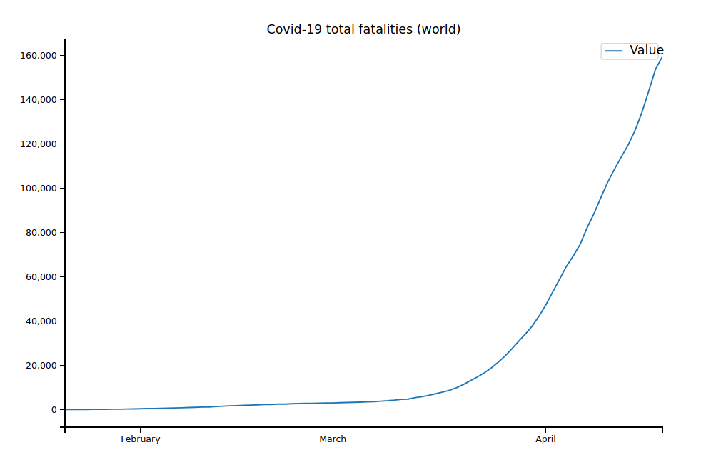
Not all countries and regions are included in the table. We can notice that we’re only using data for the number of deaths and not the number of cases reported. The reason is simple: Reporting of confirmed cases is extremely noisy and strongly depends on the number of tests (and still with enough tests, not everyone that’s infected will be getting tested). For example, the case number might increase from 10000 to 15000 from one day to the next, but that could just be because the number of tests increased by 5000. In general, the number of deaths reported is much more accurate — deaths are quite hard to miss, so the reported numbers are probably quite close to the real numbers.
Coding the Model
def deriv(y, t, beta, gamma, sigma, N, p_I_to_C, p_C_to_D, Beds):
    S, E, I, C, R, D = y

    dSdt = -beta(t) * I * S / N
    dEdt = beta(t) * I * S / N - sigma * E
    dIdt = sigma * E - 1/12.0 * p_I_to_C * I - gamma * (1 - p_I_to_C) * I
    dCdt = 1/12.0 * p_I_to_C * I - 1/7.5 * p_C_to_D * min(Beds(t), C) - max(0, C-Beds(t)) - (1 - p_C_to_D) * 1/6.5 * min(Beds(t), C)
    dRdt = gamma * (1 - p_I_to_C) * I + (1 - p_C_to_D) * 1/6.5 * min(Beds(t), C)
    dDdt = 1/7.5 * p_C_to_D * min(Beds(t), C) + max(0, C-Beds(t))
    return dSdt, dEdt, dIdt, dCdt, dRdt, dDdt
One caveat: we are calculating $\beta$ a little simplified here as calculating it rigorously would be much more complicated and would have negligible impact on the outcome.
That’s really just the equations typed into Python, nothing exciting going on! Now, onto the $R_0$-function and the whole model that takes the parameters to fit to calculate the curves of S, E, I, C, R, and D:
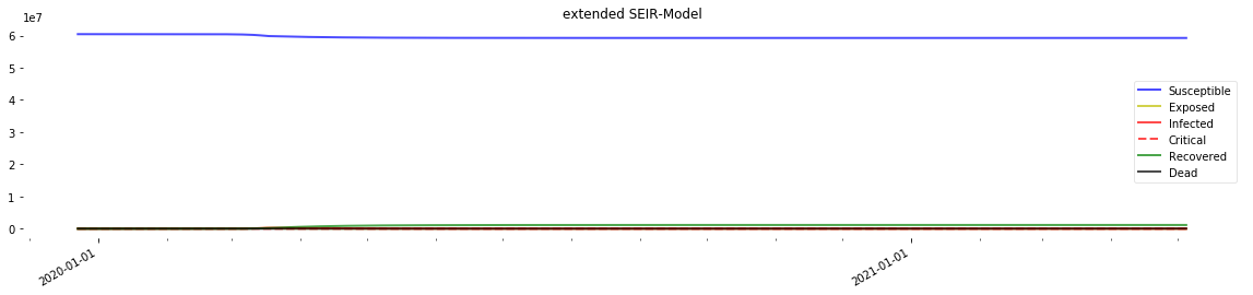
Here’s what we get when we simulate a disease in a population with not enough ICU beds
gamma = 1.0/9.0
sigma = 1.0/3.0

def logistic_R_0(t, R_0_start, k, x0, R_0_end):
    return (R_0_start-R_0_end) / (1 + np.exp(-k*(-t+x0))) + R_0_end

def Model(days, agegroups, beds_per_100k, R_0_start, k, x0, R_0_end, prob_I_to_C, prob_C_to_D, s):

    def beta(t):
        return logistic_R_0(t, R_0_start, k, x0, R_0_end) * gamma

    # agegroups is list with number of people per age group -> sum to get population
    N = sum(agegroups)

    def Beds(t):
        # the table stores beds per 100 k -> get total number
        beds_0 = beds_per_100k / 100_000 * N
        return beds_0 + s*beds_0*t  # 0.003

    y0 = N-1.0, 1.0, 0.0, 0.0, 0.0, 0.0  # one exposed, everyone else susceptible
    t = np.linspace(0, days, days)
    ret = odeint(deriv, y0, t, args=(beta, gamma, sigma, N, prob_I_to_C, prob_C_to_D, Beds))
    S, E, I, C, R, D = ret.T

    R_0_over_time = [beta(i)/gamma for i in range(len(t))]  # get R0 over time for plotting

    return t, S, E, I, C, R, D, R_0_over_time, Beds, prob_I_to_C, prob_C_to_D


plt.gcf().subplots_adjust(bottom=0.15)

def plotter(t, S, E, I, C, R, D, R_0, B, S_1=None, S_2=None, x_ticks=None):
    if S_1 is not None and S_2 is not None:
          print(f"percentage going to ICU: {S_1*100}; percentage dying in ICU: {S_2 * 100}")


    f, ax = plt.subplots(1,1,figsize=(20,4))
    if x_ticks is None:
        ax.plot(t, S, 'b', alpha=0.7, linewidth=2, label='Susceptible')
        ax.plot(t, E, 'y', alpha=0.7, linewidth=2, label='Exposed')
        ax.plot(t, I, 'r', alpha=0.7, linewidth=2, label='Infected')
        ax.plot(t, C, 'r--', alpha=0.7, linewidth=2, label='Critical')
        ax.plot(t, R, 'g', alpha=0.7, linewidth=2, label='Recovered')
        ax.plot(t, D, 'k', alpha=0.7, linewidth=2, label='Dead')
    else:
        ax.plot(x_ticks, S, 'b', alpha=0.7, linewidth=2, label='Susceptible')
        ax.plot(x_ticks, E, 'y', alpha=0.7, linewidth=2, label='Exposed')
        ax.plot(x_ticks, I, 'r', alpha=0.7, linewidth=2, label='Infected')
        ax.plot(x_ticks, C, 'r--', alpha=0.7, linewidth=2, label='Critical')
        ax.plot(x_ticks, R, 'g', alpha=0.7, linewidth=2, label='Recovered')
        ax.plot(x_ticks, D, 'k', alpha=0.7, linewidth=2, label='Dead')

        ax.xaxis.set_major_locator(mdates.YearLocator())
        ax.xaxis.set_major_formatter(mdates.DateFormatter('%Y-%m-%d'))
        ax.xaxis.set_minor_locator(mdates.MonthLocator())
        f.autofmt_xdate()


    ax.title.set_text('extended SEIR-Model')

    ax.grid(b=True, which='major', c='w', lw=2, ls='-')
    legend = ax.legend()
    legend.get_frame().set_alpha(0.5)
    for spine in ('top', 'right', 'bottom', 'left'):
        ax.spines[spine].set_visible(False)

    plt.show();

    f = plt.figure(figsize=(20,4))
    # sp1
    ax1 = f.add_subplot(131)
    if x_ticks is None:
        ax1.plot(t, R_0, 'b--', alpha=0.7, linewidth=2, label='R_0')
    else:
        ax1.plot(x_ticks, R_0, 'b--', alpha=0.7, linewidth=2, label='R_0')
        ax1.xaxis.set_major_locator(mdates.YearLocator())
        ax1.xaxis.set_major_formatter(mdates.DateFormatter('%Y-%m-%d'))
        ax1.xaxis.set_minor_locator(mdates.MonthLocator())
        f.autofmt_xdate()


    ax1.title.set_text('R_0 over time')
    ax1.grid(b=True, which='major', c='w', lw=2, ls='-')
    legend = ax1.legend()
    legend.get_frame().set_alpha(0.5)
    for spine in ('top', 'right', 'bottom', 'left'):
        ax.spines[spine].set_visible(False)

    # sp2
    ax2 = f.add_subplot(132)
    total_CFR = [0] + [100 * D[i] / sum(sigma*E[:i]) if sum(sigma*E[:i])>0 else 0 for i in range(1, len(t))]
    daily_CFR = [0] + [100 * ((D[i]-D[i-1]) / ((R[i]-R[i-1]) + (D[i]-D[i-1]))) if max((R[i]-R[i-1]), (D[i]-D[i-1]))>10 else 0 for i in range(1, len(t))]
    if x_ticks is None:
        ax2.plot(t, total_CFR, 'r--', alpha=0.7, linewidth=2, label='total')
        ax2.plot(t, daily_CFR, 'b--', alpha=0.7, linewidth=2, label='daily')
    else:
        ax2.plot(x_ticks, total_CFR, 'r--', alpha=0.7, linewidth=2, label='total')
        ax2.plot(x_ticks, daily_CFR, 'b--', alpha=0.7, linewidth=2, label='daily')
        ax2.xaxis.set_major_locator(mdates.YearLocator())
        ax2.xaxis.set_major_formatter(mdates.DateFormatter('%Y-%m-%d'))
        ax2.xaxis.set_minor_locator(mdates.MonthLocator())
        f.autofmt_xdate()

    ax2.title.set_text('Fatality Rate (%)')
    ax2.grid(b=True, which='major', c='w', lw=2, ls='-')
    legend = ax2.legend()
    legend.get_frame().set_alpha(0.5)
    for spine in ('top', 'right', 'bottom', 'left'):
        ax.spines[spine].set_visible(False)

    # sp3
    ax3 = f.add_subplot(133)
    newDs = [0] + [D[i]-D[i-1] for i in range(1, len(t))]
    if x_ticks is None:
        ax3.plot(t, newDs, 'r--', alpha=0.7, linewidth=2, label='total')
        ax3.plot(t, [max(0, C[i]-B(i)) for i in range(len(t))], 'b--', alpha=0.7, linewidth=2, label="over capacity")
    else:
        ax3.plot(x_ticks, newDs, 'r--', alpha=0.7, linewidth=2, label='total')
        ax3.plot(x_ticks, [max(0, C[i]-B(i)) for i in range(len(t))], 'b--', alpha=0.7, linewidth=2, label="over capacity")
        ax3.xaxis.set_major_locator(mdates.YearLocator())
        ax3.xaxis.set_major_formatter(mdates.DateFormatter('%Y-%m-%d'))
        ax3.xaxis.set_minor_locator(mdates.MonthLocator())
        f.autofmt_xdate()

    ax3.title.set_text('Deaths per day')
    ax3.yaxis.set_tick_params(length=0)
    ax3.xaxis.set_tick_params(length=0)
    ax3.grid(b=True, which='major', c='w', lw=2, ls='-')
    legend = ax3.legend()
    legend.get_frame().set_alpha(0.5)
    for spine in ('top', 'right', 'bottom', 'left'):
        ax.spines[spine].set_visible(False)

    plt.show();

plotter(*Model(days=500, agegroups=[100000, 100000, 100000, 100000, 100000, 100000, 100000, 100000, 100000],
               beds_per_100k=50, R_0_start=4.0, k=1.0, x0=60, R_0_end=1.0,
               prob_I_to_C=0.05, prob_C_to_D=0.6, s=0.003))
percentage going to ICU: 5.0; percentage dying in ICU: 60.0


<Figure size 432x288 with 0 Axes>
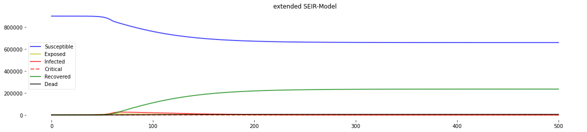
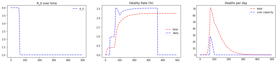
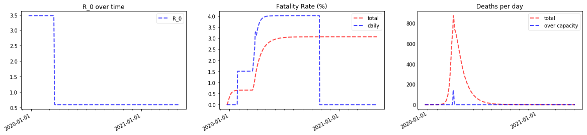
We can see the spike in deaths attributed to resource shortage (not enough beds) in the graph in the lower right corner.
Right, we now have the model and the data. Let’s put our curve fitting skills to good use!
Curve Fitting
First, we get the data to fit and the parameters we already know, and we define initial guesses and lower and upper bounds for those we do not know (to aid the curve fitter and get good results).
One parameter that’s very important and that we haven’t talked about yet is outbreak_shift: The case data begins on January 21, so our model will think that the virus started to spread on that day. For many countries, this could have in fact been days or weeks later or earlier, and it has a big impact on the fitting. Of course, we still don’t know when the first person was infected in each country — use your best judgement. For example, if you think that the country you are trying to fit had the first case on January 30, you should set outbreak_shift to -9.
(Sadly, it’s not easy to use outbreak_shift as an additional parameter as only integers (full days) are allowed, and integer programming is pretty hard (NP-hard)). We now fill up the data we want to fit (the fatalities per day) with zeroes at the beginning to account for the outbreak shift. We also define the x values for fitting; that’s just a list [0, 1, 2, …, number of days total].
For fitting, we need a function that takes exactly an x-value as first argument (the day) and all the parameters we want to fit, and that returns the deaths predicted by the model for that x-value and the parameters, so that the curve fitter can compare the model prediction to the real data. Here it is:
def fitter(x, R_0_start, k, x0, R_0_end, prob_I_to_C, prob_C_to_D, s):
    ret = Model(days, agegroups, beds_per_100k, R_0_start, k, x0, R_0_end, prob_I_to_C, prob_C_to_D, s)
    # Model returns bit tuple. 7-th value (index=6) is list with deaths per day.
    deaths_predicted = ret[6]
    return deaths_predicted[x]
# parameters
data = covid_data[covid_data["Location"] == "Italy"]["Value"].values[::-1]
agegroups = agegroup_lookup["Italy"]
beds_per_100k = beds_lookup["Italy"]
outbreak_shift = 30
params_init_min_max = {"R_0_start": (3.0, 2.0, 5.0), "k": (2.5, 0.01, 5.0), "x0": (90, 0, 120), "R_0_end": (0.9, 0.3, 3.5),
                       "prob_I_to_C": (0.05, 0.01, 0.1), "prob_C_to_D": (0.5, 0.05, 0.8),
                       "s": (0.003, 0.001, 0.01)}  # form: {parameter: (initial guess, minimum value, max value)}


days = outbreak_shift + len(data)
if outbreak_shift >= 0:
    y_data = np.concatenate((np.zeros(outbreak_shift), data))
else:
    y_data = y_data[-outbreak_shift:]

x_data = np.linspace(0, days - 1, days, dtype=int)  # x_data is just [0, 1, ..., max_days] array
There’s not much left to do! Just initialize a curve fitting model, set the parameters according to the inits, mins, and maxs we defined, set a fit method, and fit:
And — finally — here’s the fit we get for Italy:
mod = lmfit.Model(fitter)

for kwarg, (init, mini, maxi) in params_init_min_max.items():
    mod.set_param_hint(str(kwarg), value=init, min=mini, max=maxi, vary=True)

params = mod.make_params()
fit_method = "leastsq"

result = mod.fit(y_data, params, method=fit_method, x=x_data)

result.plot_fit(datafmt="-")
<matplotlib.axes._subplots.AxesSubplot at 0x1d28dfc1438>
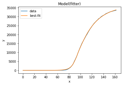
Great, they look quite realistic and in-line with many data points reported in real life! x0 is 84, so with the data beginning on January 21 and the outbreak shift set to 30 days, day 84 for our model is March 15. x0 is the date of the steepest decline in R0, so our model thinks that the main “lockdown” took place in Italy around March 15, very close to the real date.
Let’s use the best-fitting parameters to get a look at the future our model predicts
full_days = 500
first_date = np.datetime64(covid_data.Date.min()) - np.timedelta64(outbreak_shift,'D')
x_ticks = pd.date_range(start=first_date, periods=full_days, freq="D")
print("Prediction for Italy")
plotter(*Model(full_days, agegroup_lookup["Italy"], beds_lookup["Italy"], **result.best_values), x_ticks=x_ticks);
Prediction for Italy
percentage going to ICU: 7.859682796217698; percentage dying in ICU: 54.18656878713506
Note the spike in deaths due to filled hospitals around the end of march 2020 that increases the fatality rate, which finally comes out at around 1.4%.
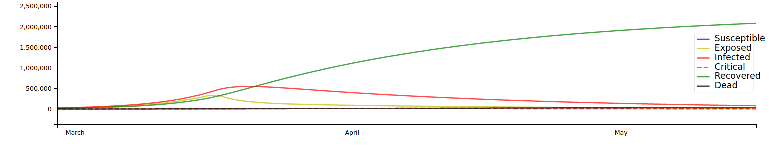
Here’s the prediction zoomed in on March to May — if the model is right, Italy has gone through the worst already and deaths should decrease strongly over the next months. Of course, our model thinks that $R_0$ will stay around 0.6; if it goes up again as lockdowns are reverted, the numbers will start increasing again!