
Introduction
AirBnB is a marketplace for short term rentals that allows you to list part or all of your living space for others to rent. You can rent everything from a room in an apartment to your entire house on AirBnB. Because most of the listings are on a short-term basis, AirBnB has grown to become a popular alternative to hotels. The company itself has grown from it’s founding in 2008 to a 30 billion dollar valuation in 2016 and is currently worth more than any hotel chain in the world.AirBnB is a marketplace for short term rentals that allows you to list part or all of your living space for others to rent. You can rent everything from a room in an apartment to your entire house on AirBnB. Because most of the listings are on a short-term basis, AirBnB has grown to become a popular alternative to hotels. The company itself has grown from it’s founding in 2008 to a 30 billion dollar valuation in 2016 and is currently worth more than any hotel chain in the world.
One challenge that hosts looking to rent their living space face is determining the optimal nightly rent price. In many areas, renters are presented with a good selection of listings and can filter on criteria like price, number of bedrooms, room type and more. Since AirBnB is a marketplace, the amount a host can charge on a nightly basis is closely linked to the dynamics of the marketplace. As a host, if we try to charge above market price for a living space we’d like to rent, then renters will select more affordable alternatives which are similar to ours. If we set our nightly rent price too low, we’ll miss out on potential revenue. One strategy we could use is to:
- find a few listings that are similar to ours,
- average the listed price for the ones most similar to ours,
- set our listing price to this calculated average price.
We want to use data on local listings to predict the optimal price for us to set. We’ll explore a specific machine learning technique called k-nearest neighbors, which mirrors the strategy we just described. Before we dive further into machine learning and k-nearest neighbors, let’s get familiar with the dataset we’ll be working with.
While AirBnB doesn’t release any data on the listings in their marketplace, a separate group named Inside AirBnB has extracted data on a sample of the listings for many of the major cities on the website. We’ll be working with their dataset from October 23, 2015 on the listings from Washington, D.C., the capital of the United States. Here’s a direct link to that dataset. Each row in the dataset is a specific listing that’s available for renting on AirBnB in the Washington, D.C. area.
To make the dataset less cumbersome to work with, some of the columns have been removed from the original dataset and renamed the file to dc_airbnb.csv. Here is a list of available columns:
- host_response_rate: the response rate of the host
- host_acceptance_rate: number of requests to the host that convert to rentals
- host_listings_count: number of other listings the host has
- latitude: latitude dimension of the geographic coordinates
- longitude: longitude part of the coordinates
- city: the city the living space resides
- zipcode: the zip code the living space resides
- state: the state the living space resides
- accommodates: the number of guests the rental can accommodate
- room_type: the type of living space (Private room, Shared room or Entire home/apt
- bedrooms: number of bedrooms included in the rental
- bathrooms: number of bathrooms included in the rental
- beds: number of beds included in the rental
- price: nightly price for the rental
- cleaning_fee: additional fee used for cleaning the living space after the guest leaves
- security_deposit: refundable security deposit, in case of damages
- minimum_nights: minimum number of nights a guest can stay for the rental
- maximum_nights: maximum number of nights a guest can stay for the rental
- number_of_reviews: number of reviews that previous guests have left
Let’s read the dataset into Pandas and become more familiar with it.
import pandas as pd

dc_listings = pd.read_csv('dc_airbnb.csv')
dc_listings.head()
| host_response_rate | host_acceptance_rate | host_listings_count | accommodates | room_type | bedrooms | bathrooms | beds | price | cleaning_fee | security_deposit | minimum_nights | maximum_nights | number_of_reviews | latitude | longitude | city | zipcode | state |
|---|---|---|---|---|---|---|---|---|---|---|---|---|---|---|---|---|---|---|
| 92% | 91% | 26 | 4 | Entire home/apt | 1 | 1 | 2 | $160.00 | $115.00 | $100.00 | 1 | 1125 | 0 | 38.89004639 | -77.0028081 | Washington | 20003 | DC |
| 90% | 100% | 1 | 6 | Entire home/apt | 3 | 3 | 3 | $350.00 | $100.00 | 2 | 30 | 65 | 38.88041282 | -76.99048487 | Washington | 20003 | DC | |
| 90% | 100% | 2 | 1 | Private room | 1 | 2 | 1 | $50.00 | 2 | 1125 | 1 | 38.95529092 | -76.98600574 | Hyattsville | 20782 | MD |
dc_listings.info()
<class 'pandas.core.frame.DataFrame'>
RangeIndex: 3723 entries, 0 to 3722
Data columns (total 19 columns):
host_response_rate      3289 non-null object
host_acceptance_rate    3109 non-null object
host_listings_count     3723 non-null int64
accommodates            3723 non-null int64
room_type               3723 non-null object
bedrooms                3702 non-null float64
bathrooms               3696 non-null float64
beds                    3712 non-null float64
price                   3723 non-null object
cleaning_fee            2335 non-null object
security_deposit        1426 non-null object
minimum_nights          3723 non-null int64
maximum_nights          3723 non-null int64
number_of_reviews       3723 non-null int64
latitude                3723 non-null float64
longitude               3723 non-null float64
city                    3723 non-null object
zipcode                 3714 non-null object
state                   3723 non-null object
dtypes: float64(5), int64(5), object(9)
memory usage: 552.7+ KB
Data Cleaning
Before we proceed, we need to clean the price column. Right now, the price column contains comma characters (,) and dollar sign characters and is formatted as a text column instead of a numeric one. We need to remove these values and convert the entire column to the float datatype.
# Cleaning the price column
price = dc_listings['price'].str.replace(',','').str.replace('$','').astype(float)
dc_listings['price'] = price
The following columns contain non-numerical values:
- room_type: e.g. Private room
- city: e.g. Washington
- state: e.g. DC
while these columns contain numerical but non-ordinal values:
- latitude: e.g. 38.913458
- longitude: e.g. -77.031
- zipcode: e.g. 20009
Geographic values like these aren’t ordinal, because a smaller numerical value doesn’t directly correspond to a smaller value in a meaningful way. For example, the zip code 20009 isn’t smaller or larger than the zip code 75023 and instead both are unique, identifier values. Latitude and longitude value pairs describe a point on a geographic coordinate system and different equations are used in those cases (e.g. haversine).
While we could convert the host_response_rate and host_acceptance_rate columns to be numerical (right now they’re object data types and contain the % sign), these columns describe the host and not the living space itself. Since a host could have many living spaces and we don’t have enough information to uniquely group living spaces to the hosts themselves, let’s avoid using any columns that don’t directly describe the living space or the listing itself:
- host_response_rate
- host_acceptance_rate
- host_listings_count
Let’s remove these 9 columns from the Dataframe.
# Dropping the variables redundant for our analysis
dc_listings = dc_listings.drop(['room_type', 'city', 'state', 'latitude', 'longitude', 'zipcode', 'host_acceptance_rate', 'host_listings_count', 'host_response_rate'], axis = 1)
Of the remaining columns, 3 columns have a few missing values (less than 1% of the total number of rows):
- bedrooms
- bathrooms
- beds
Since the number of rows containing missing values for one of these 3 columns is low, we can select and remove those rows without losing much information. There are also 2 columns that have a large number of missing values:
- cleaning_fee - 37.3% of the rows
- security_deposit - 61.7% of the rows
and we can’t handle these easily. We can’t just remove the rows containing missing values for these 2 columns because we’d miss out on the majority of the observations in the dataset. Instead, let’s remove these 2 columns entirely from consideration.
# Dropping the variables with too many missing values
dc_listings = dc_listings.drop(['cleaning_fee', 'security_deposit'], axis = 1)
dc_listings = dc_listings.dropna(axis = 0)
dc_listings.isna().sum()
accommodates         0
bedrooms             0
bathrooms            0
beds                 0
price                0
minimum_nights       0
maximum_nights       0
number_of_reviews    0
dtype: int64
| accommodates | bedrooms | bathrooms | beds | price | minimum_nights | maximum_nights | number_of_reviews | |
|---|---|---|---|---|---|---|---|---|
| 4 | 1.0 | 1.0 | 2.0 | 160.0 | 1 | 1125 | 0 | |
| 6 | 3.0 | 3.0 | 3.0 | 350.0 | 2 | 30 | 65 | |
| 1 | 1.0 | 2.0 | 1.0 | 50.0 | 2 | 1125 | 1 | |
| 2 | 1.0 | 1.0 | 1.0 | 95.0 | 1 | 1125 | 0 | |
| 4 | 1.0 | 1.0 | 1.0 | 50.0 | 7 | 1125 | 0 |
while the accommodates, bedrooms, bathrooms, beds, and minimum_nights columns hover between 0 and 12 (at least in the first few rows), the values in the maximum_nights and number_of_reviews columns span much larger ranges. For example, the maximum_nights column has values as low as 4 and high as 1825, in the first few rows itself. If we use these 2 columns as part of a k-nearest neighbors model, these attributes could end up having an outsized effect on the distance calculations because of the large values.
For example, 2 living spaces could be identical across every attribute but be vastly different just on the maximum_nights column. If one listing had a maximum_nights value of 1825 and the other a maximum_nights value of 4, because of the way Euclidean distance is calculated, these listings would be considered very far apart because of the outsized effect the largeness of the values had on the overall Euclidean distance. To prevent any single column from having too much of an impact on the distance, we can normalize all of the columns to have a mean of 0 and a standard deviation of 1. Normalizing the values in each column to the standard normal distribution (mean of 0, standard deviation of 1) preserves the distribution of the values in each column while aligning the scales.
 # Normalizing the dataset
normalized_listings = (dc_listings - dc_listings.mean()) / (dc_listings.std())


normalized_listings['price'] = dc_listings['price']
normalized_listings.head(3)
| accommodates | bedrooms | bathrooms | beds | price | minimum_nights | maximum_nights | number_of_reviews | |
|---|---|---|---|---|---|---|---|---|
| 0.401366 | -0.249467 | -0.439151 | 0.297345 | 160.0 | -0.341375 | -0.016573 | -0.516709 | |
| 1.399275 | 2.129218 | 2.969147 | 1.141549 | 350.0 | -0.065038 | -0.016603 | 1.706535 | |
| -1.095499 | -0.249467 | 1.264998 | -0.546858 | 50.0 | -0.065038 | -0.016573 | -0.482505 |
K-Nearest Neighbors Model
We can start with a single feature and increase the number of features to check the accuracy using different variables. Let’s start with some univariate k-nearest neighbors models. Starting from simple models before moving to complex model helps in structuring code workflow. Let’s create a function knn_train_test() that encapsulates the training and simple validation process. This function takes in three parameters – training column name, target column name, and the dataframe object. This function will split the data set into a training and test set. Then, it will instantiate the KNeighborsRegressor class, fit the model on the training set, and make predictions on the test set. Finally, it will calculate the RMSE and return that value.
from sklearn.neighbors import KNeighborsRegressor
from sklearn.metrics import mean_squared_error


def knn_train_test(X, target, df):

    np.random.seed(1)

    # Randomize order of rows in data frame.
    shuffled_index = np.random.permutation(df.index)
    rand_df = df.reindex(shuffled_index)

    # Divide number of rows in half and round.
    train_rows = int(len(rand_df) / 2)
    train_df = rand_df.iloc[0:train_rows]
    test_df = rand_df.iloc[train_rows:]

    # Fit a knn model and make predictions
    knn = KNeighborsRegressor()
    knn.fit(train_df[[X]], train_df[target])
    predictions = knn.predict(test_df[[X]])

    # Calculate the mse and rmse
    mse = mean_squared_error(test_df[target], predictions)
    rmse = np.sqrt(mse)

    return rmse
uni_rmse = {}

for i in normalized_listings:
    if i != 'price':
        uni_rmse[i] = knn_train_test(i, 'price', normalized_listings)

# Create a Series object from the dictionary so
# we can easily view the results, sort, etc
uni_rmse = pd.Series(uni_rmse)
uni_rmse.sort_values()
The table below shows the RMSE values of all the features when they are considered individually to predict the price of the listing.
| Features | RMSE |
|---|---|
| accommodates | 127.483339 |
| bathrooms | 128.08823 |
| beds | 133.205746 |
| bedrooms | 139.232119 |
| minimum_nights | 140.7557 |
| maximum_nights | 141.992181 |
| number_of_reviews | 174.605384 |
Let’s modify the knn_train_test() function to accept a list of column names and modify the rest of the function logic to use this parameter:
- Instead of using just a single column for train and test, use all of the columns passed in.
- Use a the default k value from scikit-learn.
def knn_train_test(X, target, df):

    np.random.seed(1)

    # Randomize order of rows in data frame.
    shuffled_index = np.random.permutation(df.index)
    rand_df = df.reindex(shuffled_index)

    # Divide number of rows in half and round.
    train_rows = int(len(rand_df) / 2)
    train_df = rand_df.iloc[0:train_rows]
    test_df = rand_df.iloc[train_rows:]

    # Fit a knn model and make predictions
    knn = KNeighborsRegressor()
    knn.fit(train_df[X], train_df[target])
    predictions = knn.predict(test_df[X])

    # Calculate the mse and rmse
    mse = mean_squared_error(test_df[target], predictions)
    rmse = np.sqrt(mse)

    return rmse
Let’s train the multi-variate model utilizing different features based on the RMSE values listed in the table above.
k_rmse_multi_results = {}


two_best_features = ['accommodates', 'bathrooms']
rmse_val = knn_train_test(two_best_features, 'price', normalized_listings)
k_rmse_multi_results["two best features"] = rmse_val

three_best_features = ['accommodates', 'bathrooms', 'beds']
rmse_val = knn_train_test(three_best_features, 'price', normalized_listings)
k_rmse_multi_results["three best features"] = rmse_val

four_best_features = ['accommodates', 'bathrooms', 'beds', 'bedrooms']
rmse_val = knn_train_test(four_best_features, 'price', normalized_listings)
k_rmse_multi_results["four best features"] = rmse_val

five_best_features = ['accommodates', 'bathrooms', 'beds', 'bedrooms', 'minimum_nights']
rmse_val = knn_train_test(five_best_features, 'price', normalized_listings)
k_rmse_multi_results["five best features"] = rmse_val

six_best_features = ['accommodates', 'bathrooms', 'beds', 'bedrooms', 'minimum_nights', 'maximum_nights']
rmse_val = knn_train_test(six_best_features, 'price', normalized_listings)
k_rmse_multi_results["six best features"] = rmse_val

k_rmse_multi_results
{'five best features': 121.29424844518537,
 'four best features': 130.45776727122973,
 'six best features': 125.63507413080096,
 'three best features': 133.14108206787563,
 'two best features': 126.89462880347659}
Hyperparameter Optimization
When we focused on increasing the number of attributes we saw how, in general, adding more attributes generally lowered the error of the model. This is because the model is able to do a better job identifying the living spaces from the training set that are the most similar to the ones from the test set. However, we also observed how using all of the available features didn’t actually improve the model’s accuracy automatically and that some of the features were probably not relevant for similarity ranking. We learned that selecting relevant features was the right lever when improving a model’s accuracy, not just increasing the features used in the absolute.
When we vary the features that are used in the model, we’re affecting the data that the model uses. On the other hand, varying the k value affects the behavior of the model independently of the actual data that’s used when making predictions. In other words, we’re impacting how the model performs without trying to change the data that’s used.
Values that affect the behavior and performance of a model that are unrelated to the data that’s used are referred to as hyperparameters. The process of finding the optimal hyperparameter value is known as hyperparameter optimization. A simple but common hyperparameter optimization technique is known as grid search, which involves:
- selecting a subset of the possible hyperparameter values,
- training a model using each of these hyperparameter values,
- evaluating each model’s performance,
- selecting the hyperparameter value that resulted in the lowest error value.
Grid search essentially boils down to evaluating the model performance at different k values and selecting the k value that resulted in the lowest error. While grid search can take a long time when working with large datasets, the data we’re working with in this project is small and this process is relatively quick. Let’s confirm that grid search will work quickly for the dataset we’re working with by first observing how the model performance changes as we increase the k value from 1 to 5
def knn_train_test(train_cols, target_col, df):
    np.random.seed(1)

    # Randomize order of rows in data frame.
    shuffled_index = np.random.permutation(df.index)
    rand_df = df.reindex(shuffled_index)

    # Divide number of rows in half and round.
    last_train_row = int(len(rand_df) / 2)

    # Select the first half and set as training set.
    # Select the second half and set as test set.
    train_df = rand_df.iloc[0:last_train_row]
    test_df = rand_df.iloc[last_train_row:]

    k_values = [x for x in range(1, 26)]
    k_rmses = {}

    for k in k_values:
        # Fit model using k nearest neighbors.
        knn = KNeighborsRegressor(n_neighbors=k)
        knn.fit(train_df[train_cols], train_df[target_col])

        # Make predictions using model.
        predicted_labels = knn.predict(test_df[train_cols])

        # Calculate and return RMSE.
        mse = mean_squared_error(test_df[target_col], predicted_labels)
        rmse = np.sqrt(mse)

        k_rmses[k] = rmse
    return k_rmses
k_rmse_multi_results = {}


two_best_features = ['accommodates', 'bathrooms']
rmse_val = knn_train_test(two_best_features, 'price', normalized_listings)
k_rmse_multi_results["two best features"] = rmse_val

three_best_features = ['accommodates', 'bathrooms', 'beds']
rmse_val = knn_train_test(three_best_features, 'price', normalized_listings)
k_rmse_multi_results["three best features"] = rmse_val

four_best_features = ['accommodates', 'bathrooms', 'beds', 'bedrooms']
rmse_val = knn_train_test(four_best_features, 'price', normalized_listings)
k_rmse_multi_results["four best features"] = rmse_val
``python import matplotlib.pyplot as plt %matplotlib inline
i = [] for k,v in k_rmse_multi_results.items(): x = list(v.keys()) y = list(v.values()) y.insert(4, y.pop(2)) i.append(k)
plt.plot(x,y)
plt.xlabel('k value')
plt.ylabel('RMSE')
plt.legend(i, loc='upper right')
```
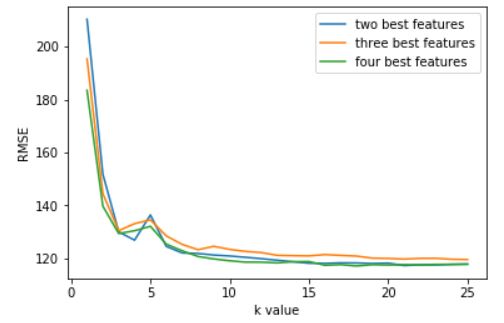
Conclusion
As we increased the k value from 1 to 8, the RMSE value decreased from approximately 210 to approximately 120. However, as we increased the k value from 9 to 25, the MSE value didn’t decrease further but instead hovered between approximately 121 and 120. This means that the optimal k value is 8, since the RMSE values don’t deviate much from 120.